📊 Lec 11 -

This lesson builds core statistical understanding for BSc Agriculture exam preparation through clear concepts, worked structures, and application-focused interpretation.

---

Attributes

Contingency table – 2x2 contingency table – Test for independence of attributes – test for goodness of fit of mendalian ratio

Test based on -distribution

In case of attributes we can not employ the parametric tests such as F and t. Instead we have to apply test. When we want to test whether a set of observed values are in agreement with those expected on the basis of some theories or hypothesis. The statistic provides a measure of agreement between such observed and expected frequencies.

Chi-Square

The test has a number of applications. It is used to

• Test the independence of attributes
• Test the goodness of fit
• Test the homogeneity of variances
• Test the homogeneity of correlation coefficients
• Test the equaslity of several proportions.

In genetics it is applied to detect linkage.

Applications

– test for goodness of fit

A very powerful test for testing the significance of the discrepancy between theory and experiment was given by Prof. Karl Pearson in 1900 and is known as “chi-square test of goodness of fit “.

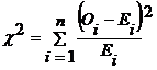
If 0i, (i=1,2,…..,n) is a set of observed (experimental frequencies) and Ei (i=1,2,…..,n) is the corresponding set of expected (theoretical or hypothetical) frequencies, then, It follows a **distribution with n-1 d.f. In case of**only one tailed test is used.

Example

In plant genetics, our interest may be to test whether the observed segregation ratios deviate significantly from the mendelian ratios. In such situations we want to test the agreement between the observed and theoretical frequency, such test is called as test of goodness of fit.

Conditions for the validity of -test: -test is an approximate test for large values of ‘n’ for the validity of -test of goodness of fit between theory and experiment, the following conditions must be satisfied.

• The sample observations should be independent.

2. Constraints on the cell freqrequency, if any, should be linear. Example:=.

3. N, the total frequency should be reasonably large, say greater then (>) 50.

4. No theoretical cell frequency should be less than (<)5. If any theoretical cell frequency is <5, then for the application of - test, it is pooled with the preceding or scecceeding frequency so that the pooled frequency is more than 5 and finally adjust for degree’s of freedom lost in pooling.

Example1

The number of yiest cells counted in a haemocytometer is compared to the theoretical value is given below. Does the experimental result support the theory?

No. of Yeast cells in the square	Obseved Frequency	Expected Frequency
0	103	106
1	143	141
2	98	93
3	42	41
4	8	14
5	6	5

Solution

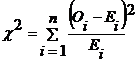
H0: the experimental results support the theory H1: the esperimental results does not support the theory. Level of significance=5% Test Statistic:

Oi | Ei | Oi­-Ei | (Oi­-Ei)2 | (Oi­-Ei)2/Ei

---|---|---|---|--- 103 | 106 | -3 | 9 | 0.0849 143 | 141 | 2 | 4 | 0.0284 98 | 93 | 5 | 25 | 0.2688 42 | 41 | 1 | 1 | 0.0244 8 | 14 | -6 | 36 | 2.5714 6 | 5 | 1 | 1 | 0.2000 400 | 400 | | | 3.1779

****=3.1779

Table value

(6-1=5 at 5 % l.os)= 11.070 Inference < tab We accept the null hypothesis. (i.e) there is a good correspondence between theory and experiment.

test for independence of attributes

At times we may consider two charactertistics on attributes simultaneously. Our interest will be to test the association between these two attributes Example :- An entomologist may be interested to know the effectiveness of different concentrations of the chemical in killing the insects. The concentrations of chemical form one attribute. The state of insects ‘killed & not killed’ forms another attribute. The result of this experiment can be arranged in the form of a contingency table. In general one attribute may be divided into m classes as A 1,A 2, …….A m and the other attribute may be divided into n classes as B 1,B 2, ……B n . Then the contingency table will have m x n cells. It is termed as m x n contingency table

A

B	A1	A2	…	Aj	…	Am	Row Total
B1	O11	O12	…	O1j		O1m	r1
B2	O21	O22	…	O2j		O2m	r2
.
.
.
Bi	Oij	Oi2	…	Oij		Oim	ri
.
.
.
Bn	On1	On2	…	Onj		Onm	rk
Column Total	c1	c2	…	cj	…	cm	n=

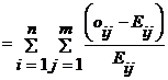
where Oij’s are observed frequencies. The expected frequencies corresponding to Oij is calculated as . The is computed as where Oij – observed frequencies Eij – Expected frequencies n= number of rows m= number of columns It can be verified that This is distributed as with (n-1) (m-1) d.f.

2x2 – contingency table

When the number of rows and numberof columns are equal to 2 it is termed as 2 x 2 contingency table .It will be in the following form

| B1 B2 | Row Total ---|---|--- A1 A2 | a b c d | a+b r1 c+d r2 Column Total | a+c b+d c1 c2 | a+b+c+d =n

Where a, b, c and d are cell frequancies c1 and c2 are column totals, r1 and r2 are row totals and n is the total number of observations. In case of 2 x 2 contigency table can be directly found using the short cut formula, The d.f associated with is (2-1) (2-1) =1

Yates correction for continuity

If anyone of the cell frequency is < 5, we use Yates correction to make as continuous. The yares correction is made by adding 0.5 to the least cell frequency and adjusting the other cell frequencies so that the column and row totals remain same . suppose, the firat cell frequency is to be corrected then the consigency table will be as follows:

| B1 | B2 | Row Total ---|---|---|--- A1 A2 | a | b | a+b=r1 c | d | c+d =r2 Column Total | a+c=c1 | b+d=c2 | n = a+b+c+d

Then use the - statistic as

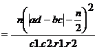The d.f associated with is (2-1) (2-1) =1

Exapmle 2

The severity of a disease and blood group were studied in a research projest. The findings sre given in the following table, knowmn as the m xn contingency table. Can this severity of the condition and blood group are associated. Severity of a disease classified by blood group in 1500 patients.

Condition	Blood Groups	Total
O	A	B
Severe	51	40
Moderate	105	103
Mild	384	527
Total	540	670

Solution

H0: The severity of the disease is not associated with blood group. H1: The severity of the disease is associated with blood group. Calculation of Expected frequencies

Condition	Blood Groups	Total
O	A	B
Severe	39.6	49.1
Moderate	90.0	111.7
Mild	410.4	509.2
Total	540	670

Test statistic: 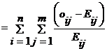The d.f. associated with the is (3-1)(4-1) = 6

Calculations

Oi | Ei | Oi­-Ei | (Oi­-Ei)2 | (Oi­-Ei)2/Ei

---|---|---|---|--- 51 | 39.6 | 11.4 | 129.96 | 3.2818 40 | 49.1 | -9.1 | 82.81 | 1.6866 10 | 11.7 | -1.7 | 2.89 | 0.2470 9 | 9.5 | -0.5 | 0.25 | 0.0263 105 | 90.0 | 15 | 225.00 | 2.5000 103 | 111.7 | -8.7 | 75.69 | 0.6776 25 | 26.7 | -1.7 | 2.89 | 0.1082 17 | 21.7 | -4.7 | 22.09 | 1.0180 384 | 410.4 | -26.4 | 696.96 | 1.6982 527 | 509.2 | 17.8 | 316.84 | 0.6222 125 | 121.6 | 3.4 | 11.56 | 0.0951 104 | 98.8 | 5.2 | 27.04 | 0.2737 Total | 12.2347

****=12.2347 Table value of for 6 d.f. at 5% level of significance is 12.59 Inference < tab We accept the null hypothesis. The severity of the disease has no association with blood group.

Example 3

In order to determine the possible effect of a chemical treatment on the rate of germination of cotton seeds a pot culture experiment was conducted. The results are given below Chemical treatment and germination of cotton seeds

| Germinated | Not germinated | Total ---|---|---|--- Chemically Treated | 118 | 22 | 140 Untreated | 120 | 40 | 160 Total | 238 | 62 | 300

Does the chemical treatrment improve the germination rate of cotton seeds?

Solution

H0:The chemical treatment does not improve the germination rate of cotton seeds. H1: The chemical treatment improves the germination rate of cotton seeds. Level of significance = 1% Test statistic

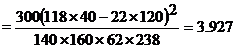
Table value

(1) d.f. at 1 % L.O.S = 6.635 Inference < tab We accept the null hypothesis. The chemical treatmentwill not improve the germination rate of cotton seeds significantly.

Example 4

In an experiment on the effect of a growth regulator on fruit setting in muskmelon the following results were obtained. Test whether the fruit setting in muskmelon and the application of growth regulator are independent at 1% level.

| Fruit set | Fruit not set | Total ---|---|---|--- Treated | 16 | 9 | 25 Control | 4 | 21 | 25 Total | 20 | 30 | 50

Solution

H0:Fruit setting in muskmelon does not depend on the application of growth regulator. H1: Fruit setting in muskmelon depend on the application of growth regulator. Level of significance = 1% After Yates correction we have

| Fruit set | Fruit not set | Total ---|---|---|--- Treated | 15.5 | 9.5 | 25 Control | 4.5 | 20.5 | 25 Total | 20 | 30 | 50

Tet statistic

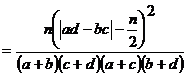
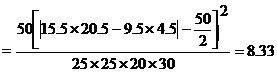
Table value

(1) d.f. at 1 % level of significance is 6.635 Inference > tab We reject the null hypothesis. Fruit setting in muskmelon is influenced by the growth regulator. Application of growth regulator will increase fruit setting in musk melon.

---|---

Summary Cheat Sheet

• Focus: core definitions, classification logic, and design/analysis workflow from this lesson.
• Exam Use: revise key terms, assumptions, and interpretation steps for objective and descriptive questions.
• Practice: solve one representative numerical or conceptual question from this topic.

References

1 source • [1]

[1]

Standard BSc Agriculture Statistics notes used for lesson preparation.