💻 Increasing & Decreasing

This lesson covers core applied mathematics concepts and their agricultural applications for BSc Agriculture learners.

---

MATHS :: Lecture 09 ::Increasing & Decreasing ,Maxima & Minima Function

Chain Rule differentiation If y is a function of u ie y = f(u) and u is a function of x ie u = g(x) then y is related to x through the intermediate function u ie y =f(g(x) ) \y is differentiable with respect to x Furthermore, let y=f(g(x)) and u=g(x), then = There are a number of related results that also go under the name of "chain rules." For example, if y=f(u) u=g(v), and v=h(x), then =

Problem

Differentiate the following with respect to x

• y = (3x2+4)3
• y =

Marginal Analysis

Let us assume that the total cost C is represented as a function total output q. (i.e) C= f(q). Then marginal cost is denoted by MC= The average cost = Similarly if U = u(x) is the utility function of the commodity x then the marginal utility MU = The total revenue function TR is the product of quantity demanded Q and the price P per unit of that commodity then TR = Q.P = f(Q) Then the marginal revenue denoted by MR is given by The average revenue =

Problem

1. If the total cost function is C = Q3 - 3Q2 + 15Q. Find Marginal cost and average cost.

Solution

MC = AC = 2. The demand function for a commodity is P= (a - bQ). Find marginal revenue. (the demand function is generally known as Average revenue function). Total revenue TR = P.Q = Q. (a - bQ) and marginal revenue MR=

Growth rate and relative growth rate

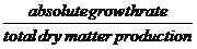
The growth of the plant is usually measured in terms of dry mater production and as denoted by W. Growth is a function of time t and is denoted by W=g(t) it is called a growth function. Here t is the independent variable and w is the dependent variable. The derivative is the growth rate (or) the absolute growth rate gr=. GR = The relative growth rate i.e defined as the absolute growth rate divided by the total dry matter production and is denoted by RGR. i.e RGR = . =

Problem

1. If G = at2+b sin t +5 is the growth function function the growth rate and relative growth rate.

GR = RGR = .

Implicit Functions

If the variables x and y are related with each other such that f (x, y) = 0 then it is called Implicit function. A function is said to be explicit when one variable can be expressed completely in terms of the other variable. For example, y = x3 + 2x2 + 3x + 1 is an Explicit function xy2 + 2y +x = 0 is an implicit function

** **

Problem

For example, the implicit equation xy=1 can be solved by differentiating implicitly gives = Implicit differentiation is especially useful when y’(x)is needed, but it is difficult or inconvenient to solve for y in terms of x. Example:__Differentiate the following function with respect to x

Solution

So, just differentiate as normal and tack on an appropriate derivative at each step. Note as well that the first term will be a product rule. Example:__ Find for the following function.

Solution

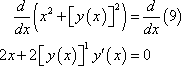
In this example we really are going to need to do implicit differentiation of x and write y as y(x). Notice that when we differentiated the y term we used the chain rule. Example:__ Find for the following. Solutio: First differentiate both sides with respect to x and notice that the first time on left side will be a product rule. Remember that very time we differentiate a y we also multiply that term by since we are just using the chain rule. Now solve for the derivative.

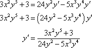
The algebra in these can be quite messy so be careful with that. Example: Find for the following Here we’ve got two product rules to deal with this time. Notice the derivative tacked onto the secant. We differentiated a y to get to that point and so we needed to tack a derivative on. Now, solve for the derivative.

Logarithmic Differentiation

For some problems, first by taking logarithms and then differentiating,

it is easier to find . Such process is called Logarithmic differentiation.

• If the function appears as a product of many simple functions then by

taking logarithm so that the product is converted into a sum. It is now easier to differentiate them.

• If the variable x occurs in the exponent then by taking logarithm it is

reduced to a familiar form to differentiate. ExampleBegin();Example Differentiate the function. MPSetEqnAttrs('eq0001','',3,[[100,34,16,-1,-1],[133,45,21,-1,-1],[166,56,26,-1,-1],[],[],[],[415,139,67,-3,-3]]) MPEqu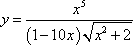ation() MPSetEqnAttrs('eq0001','',3,[[100,34,16,-1,-1],[133,45,21,-1,-1],[166,56,26,-1,-1],[],[],[],[415,139,67,-3,-3]]); Solution Differentiating this function could be done with a product rule and a quotient rule. We can simplify things somewhat by taking logarithms of both sides. MPSetEqnAttrs('eq0002','',3,[[134,40,17,-1,-1],[177,53,22,-1,-1],[221,67,29,-1,-1],[],[],[],[554,165,70,-3,-3]]) MPEquation() 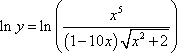MPSetEqnAttrs('eq0002','',3,[[134,40,17,-1,-1],[177,53,22,-1,-1],[221,67,29,-1,-1],[],[],[],[554,165,70,-3,-3]]); MPSetEqnAttrs('eq0003','',3,[[190,49,22,-1,-1],[253,67,30,-1,-1],[316,84,37,-1,-1],[],[],[],[792,215,95,-3,-3]]) MPEquation()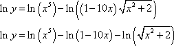 MPSetEqnAttrs('eq0003','',3,[[190,49,22,-1,-1],[253,67,30,-1,-1],[316,84,37,-1,-1],[],[],[],[792,215,95,-3,-3]]); MPSetEqnAttrs('eq0004','',3,[[175,89,42,-1,-1],[233,118,55,-1,-1],[291,148,69,-1,-1],[],[],[],[729,368,173,-3,-3]]) MPEquation()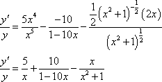 ExampleBegin(); Example Differentiate MPSetEqnAttrs('eq0007','',3,[[30,11,3,-1,-1],[39,15,3,-1,-1],[47,17,3,-1,-1],[],[],[],[119,44,9,-3,-3]]) MPEquation() MPSetEqnAttrs('eq0007','',3,[[30,11,3,-1,-1],[39,15,3,-1,-1],[47,17,3,-1,-1],[],[],[],[119,44,9,-3,-3]]); Solution First take the logarithm of both sides as we did in the first example and use the logarithm properties to simplify things a little. MPSetEqnAttrs('eq0009','',3,[[54,30,13,-1,-1],[73,39,16,-1,-1],[90,48,20,-1,-1],[],[],[],[227,120,52,-3,-3]]) MPEquation() MPSetEqnAttrs('eq0009','',3,[[54,30,13,-1,-1],[73,39,16,-1,-1],[90,48,20,-1,-1],[],[],[],[227,120,52,-3,-3]]); Differentiate both sides using implicit differentiation. 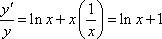MPSetEqnAttrs('eq0010','',3,[[121,30,12,-1,-1],[162,39,16,-1,-1],[203,49,20,-1,-1],[],[],[],[507,124,50,-3,-3]]) MPEquation() MPSetEqnAttrs('eq0010','',3,[[121,30,12,-1,-1],[162,39,16,-1,-1],[203,49,20,-1,-1],[],[],[],[507,124,50,-3,-3]]); As with the first example multiply by y and substitute back in for y. MPSetEqnAttrs('eq0011','',3,[[75,34,14,-1,-1],[99,45,19,-1,-1],[123,57,23,-1,-1],[],[],[],[310,145,61,-3,-3]]) MPEquation()

PARAMETRIC FUNCTIONS

Sometimes variables x and y are expressed in terms of a third variable called parameter. We find without eliminating the third variable. Let x = f(t) and y = g(t) then

= = =

Problem

1. Find for the parametric function x =a cos , y = b sin

Solution

=

= =

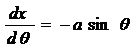
Inference of the differentiation

Let y = f(x) be a given function then the first order derivative is . The geometrical meaning of the first order derivative is that it represents the slope of the curve y = f(x) at x. The physical meaning of the first order derivative is that it represents the rate of change of y with respect to x. PROBLEMS ON HIGHER ORDER DIFFERENTIATION The rate of change of y with respect x is denoted by and called as the first order derivative of function y with respect to x. The first order derivative of y with respect to x is again a function of x, which again be differentiated with respect to x and it is called second order derivative of y = f(x) and is denoted by which is equal to In the similar way higher order differentiation can be defined. Ie. The nth order derivative of y=f(x) can be obtained by differentiating n-1th derivative of y=f(x) 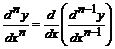where n= 2,3,4,5….

Problem

Find the first , second and third derivative of

1. y =
2. y = log(a-bx)
3. y = sin (ax+b)

Partial Differentiation

So far we considered the function of a single variable y = f(x) where x is the only independent variable. When the number of independent variable exceeds one then we call it as the function of several variables.

Example

z = f(x,y) is the function of two variables x and y , where x and y are independent variables. U=f(x,y,z) is the function of three variables x,y and z , where x, y and z are independent variables. In all these functions there will be only one dependent variable. Consider a function z = f(x,y). The partial derivative of z with respect to x denoted by and is obtained by differentiating z with respect to x keeping y as a constant. Similarly the partial derivative of z with respect to y denoted by and is obtained by differentiating z with respect to y keeping x as a constant.

Problem

1. Differentiate U = log (ax+by+cz) partially with respect to x, y & z We can also find higher order partial derivatives for the function z = f(x,y) as follows (i) The second order partial derivative of z with respect to x denoted as is obtained by partially differentiating with respect to x. this is also known as direct second order partial derivative of z with respect to x. (ii)The second order partial derivative of z with respect to y denoted as is obtained by partially differentiating with respect to y this is also known as direct second order partial derivative of z with respect to y (iii) The second order partial derivative of z with respect to x and then y denoted as is obtained by partially differentiating with respect to y. this is also known as mixed second order partial derivative of z with respect to x and then y iv) The second order partial derivative of z with respect to y and then x denoted as is obtained by partially differentiating with respect to x. this is also known as mixed second order partial derivative of z with respect to y and then x. In similar way higher order partial derivatives can be found.

Problem

Find all possible first and second order partial derivatives of

1. z = sin(ax +by)
2. u = xy + yz + zx

Homogeneous Function

A function in which each term has the same degree is called a homogeneous function.

Example

• x2 –2xy + y2 = 0 ® homogeneous function of degree 2.
• 3x +4y = 0 ® homogeneous function of degree 1.
• x3+3x2y + xy2 – y3= 0 ® homogeneous function of degree 3.

To find the degree of a homogeneous function we proceed as follows. Consider the function f(x,y) replace x by tx and y by ty if f (tx, ty) = tn f(x, y) then n gives the degree of the homogeneous function. This result can be extended to any number of variables.

Problem

Find the degree of the homogeneous function

• f(x, y) = x2 –2xy + y2
• f(x,y) =

Euler’s theorem on homogeneous function

If U= f(x,y,z) is a homogeneous function of degree n in the variables x, y & z then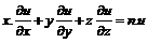

Problem

Verify Euler’s theorem for the following function 1. u(x,y) = x2 –2xy + y2 2. u(x,y) = x3 + y3+ z3–3xyz Increasing and decreasing function

Increasing function

A function y= f(x) is said to be an increasing function if f(x1) < f(x2) for all x1 < x2. The condition for the function to be increasing is that its first order derivative is always greater than zero . i.e >0

Decreasing function

A function y= f(x) is said to be a decreasing function if f(x1) > f(x2) for all x1 < x2. The condition for the function to be decreasing is that its first order derivative is always less than zero . i.e < 0

Problems

1. Show that the function y = x3 + x is increasing for all x. 2. Find for what values of x is the function y = 8 + 2x – x2 is increasing or decreasing ?

Maxima and Minima Function of a single variable

A function y = f(x) is said to have maximum at x = a if f(a) > f(x) in the neighborhood of the point x = a and f(a) is the maximum value of f(x) . The point x = a is also known as local maximum point. A function y = f(x) is said to have minimum at x = a if f(a) < f(x) in the neighborhood of the point x = a and f(a) is the minimum value of f(x) . The point x = a is also known as local minimum point. The points at which the function attains maximum or minimum are called the turning points or stationary points A function y=f(x) can have more than one maximum or minimum point . Maximum of all the maximum points is called Global maximum and minimum of all the minimum points is called Global minimum. A point at which neither maximum nor minimum is called Saddle point. [Consider a function y = f(x). If the function increases upto a particular point x = a and then decreases it is said to have a maximum at x = a. If the function decreases upto a point x = b and then increases it is said to have a minimum at a point x=b.] The necessary and the sufficient condition for the function y=f(x) to have a maximum or minimum can be tabulated as follows

| Maximum | Minimum ---|---|--- First order or necessary condition | = 0 | =0 Second order or sufficient condition | < 0 | > 0

Working Procedure

1. Find and

2. Equate =0 and solve for x. this will give the turning points of the function.

3. Consider a turning point x = a then substitute this value of x in and find the nature of the second derivative. If < 0, then the function has a maximum value at the point x = a. If > 0, then the function has a minimum value at the point x = a.

4. Then substitute x = a in the function y = f(x) that will give the maximum or minimum value of the function at x = a.

Problem

Find the maximum and minimum values of the following function

y = x3 – 3x +1

---|---

Summary Cheat Sheet

• Focus on core formulas, definitions, and solved patterns from this lesson.
• Practice stepwise derivations and numerical substitutions carefully.
• Connect each concept to practical agricultural problem-solving contexts.

References

1 source

Primary classroom notes and standard BSc Agriculture applied mathematics references.