🧣Split Plot and Strip Plot Designs

An irrigation scientist wants to test three irrigation levels and four nitrogen doses together. Irrigation requires large plots (you cannot irrigate a tiny strip differently from its neighbours), while nitrogen can be applied to smaller areas. The Split Plot Design elegantly handles this mismatch by nesting smaller sub-plots within larger main plots — each with its own precision level.

---

Split Plot Design (SPD) ^{NABARD Mains 2020}

• In field experiments certain factors may require larger plots than for others. For example, experiments on irrigation, tillage, etc. requires larger areas. On the other hand, experiments on fertilizers, etc. may not require larger areas. This practical constraint arises because some treatments (like irrigation or deep ploughing) are physically difficult to apply uniformly to small plots.

---

• To accommodate factors which require different sizes of experimental plots in the same experiment, split plot design has been evolved. SPD is essentially an extension of the Randomized Block Design (RBD) that allows two factors to be studied together, each at a different level of precision.

---

• In this design, larger plots are taken for the factor which requires larger plots. Next each of the larger plots is split into smaller plots to accommodate the other factor. The different treatments are allotted at random to their respective plots. Such arrangement is called split plot design.
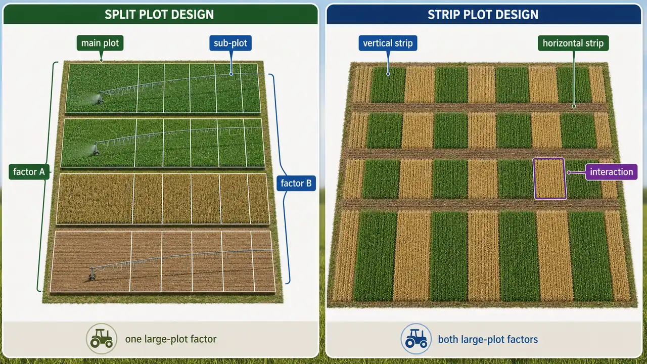
• In split plot design the larger plots are called main plots and smaller plots within the larger plots are called as sub plots.
• The factor levels allotted to the main plots are main plot treatments and the factor levels allotted to sub plots are called as sub plot treatments. An important consequence of this arrangement is that sub plot treatments are estimated with greater precision than main plot treatments, because the sub plot error is typically smaller than the main plot error.

---

👉🏻 This design used under following condition:

• When factors of the different nature are to be tested in same experiment that is level of one factor require larger area as compared to other factor e.g. Depth of ploughing and nitrogen level, date of sowing and varieties, varieties and nitrogen level, irrigation level and varieties.
• When all factors aren’t important. In this case, the less important factor is placed in main plots and the more important factor is placed in sub plots to benefit from the higher precision of sub plot comparisons.
• When all the levels of one factor produce larger differences as compared with the levels of other factors.
• When we want to study one factor with higher precision as compared to other factor and take it in sub plots (Smaller Plot).

---

ANOVA

• The analysis of variance will have two parts, which correspond to the main plots and sub-plots. This is a distinguishing feature of SPD — unlike CRD, RBD, or LSD which have a single ANOVA table, SPD has a two-part analysis with separate error terms for main plots and sub plots.

---

• For the main plot analysis, replication X main plot treatments table is formed. From this two-way table sum of squares for replication, main plot treatments and error (a) are computed. Error (a) is the main plot error, used to test the significance of main plot treatments.
• For the analysis of sub-plot treatments, main plot X sub-plot treatments table is formed.
• From this table the sums of squares for sub-plot treatments and interaction between main plot and sub-plot treatments are computed. The interaction term tells us whether the effect of one factor depends on the level of the other factor.
• Error (b) sum of squares is found out by residual method. Error (b) is the sub plot error, which is typically smaller than Error (a), providing more precise comparisons for sub plot treatments.

---

• The analysis of variance table for a split plot design with m main plot treatments and s sub-plot treatments is given below.
• Analysis of variance for split plot with factor A with m levels in main plots and factor B with s levels in sub-plots will be as follows:

• The number of error terms in a split plot design is two. This is a key fact to remember — Error (a) for testing main plot treatments and Error (b) for testing sub plot treatments and interaction.
• Error degree of freedom: m(r - 1)(s - 1)

---

SrPD (Strip Plot Design)

• This design is used when both the factors require relatively large area. Unlike SPD where only one factor needs large plots, strip plot design addresses situations where both factors demand big plot sizes.
• This design is also known as split block design. When there are two factors in an experiment and both the factors require large plot sizes it is difficult to carry out the experiment in split plot design. Also, the precision for measuring the interaction effect between the two factors is higher than that for measuring the main effect of either one of the two factors. Strip plot design is suitable for such experiments.

---

• In strip plot design each block or replication is divided into number of vertical and horizontal strips depending on the levels of the respective factors.

---

• The plot size for the treatments allotted in vertical strips will not be equal when compared to the treatments allotted in horizontal strips
• In this design there are three plot sizes. This is a unique feature — no other standard design has three different plot sizes within the same experiment.
  • Vertical strip plot for the first factor — vertical factor
  • Horizontal strip plot for the second factor — horizontal factor
  • Interaction plot for the interaction between 2 factors
• The vertical strip and the horizontal strip are always perpendicular to each other.
• The interaction plot is the smallest and provides information on the interaction of the 2 factors. Since the interaction plot is formed by the intersection of the vertical and horizontal strips, it is naturally the smallest unit, and this is why interaction is measured with the highest precision.
• Thus, we say that interaction is tested with more precision in strip plot design.

---

Analysis

• The analysis is carried out in 3 parts. Each part corresponds to one of the three plot sizes and has its own error term.
  • Vertical strip analysis
  • Horizontal strip analysis
  • Interaction analysis

---

• Suppose that A and B are the vertical and horizontal strips respectively. The following two-way tables, viz., A X Rep table, B X Rep table and A X B table are formed. From A X Rep table, SS for Rep, A and Error (a) are computed. From B X Rep table, SS for B and Error (b) are computed. From A X B table, A X B SS is calculated. Each error term is specific to its corresponding factor, allowing appropriate F-tests for each source of variation.
• When there are r replications, a level for factor A and b levels for factor B, then the ANOVA table is

• The number of error terms in a strip plot design is three. This is a crucial difference from SPD (which has two error terms) and RBD/LSD (which have one error term). The three error terms are Error (a) for factor A, Error (b) for factor B, and Error (c) for the interaction A x B.
• Error degree of freedom: (r - 1)(a - 1)(b - 1)

Quick Comparison: SPD vs Strip Plot Design

Feature	Split Plot Design (SPD)	Strip Plot Design (SrPD)
Also called	—	Split Block Design
Error terms	2 (Error a, Error b)	3 (Error a, Error b, Error c)
Plot sizes	2 (main, sub)	3 (vertical, horizontal, interaction)
Best for	Factors needing different plot sizes	Both factors need large plots
Highest precision	Sub plot treatments	Interaction effect
Use when	One factor needs larger area	Both factors need larger area

---

Summary Cheat Sheet