🥸 Testing of Hypothesis
Null and alternative hypothesis, Type I and Type II errors, degrees of freedom, level of significance, critical values, and step-by-step testing procedure
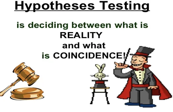
A fertiliser company claims its new product increases wheat yield by 20%. An agronomist tests it on 30 plots and finds a 15% increase. Is the difference between the claimed 20% and the observed 15% real, or could it simply be due to natural plot-to-plot variation? Hypothesis testing provides the systematic framework to answer such questions — it is the backbone of statistical inference in agricultural research.
Why Do We Need Hypothesis Testing?
- Sample estimates rarely equal the true population value due to inherent variation.
- Different samples yield different estimates. We must verify whether the difference between a sample estimate and the population value is due to sampling fluctuation or a real difference.
- If the difference is due to sampling fluctuation alone, the sample belongs to the population. If the difference is real, the sample may not belong to that population.
Key Terminology
Hypothesis
- An assumption about any unknown characteristic of a population. It may or may not be true.
- Examples: μ = 2.3, σ = 2.1, or "the population follows Normal Distribution."
- Two types: null hypothesis and alternative hypothesis.
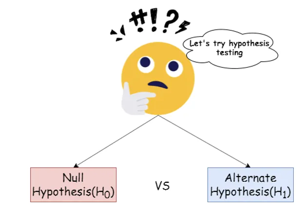
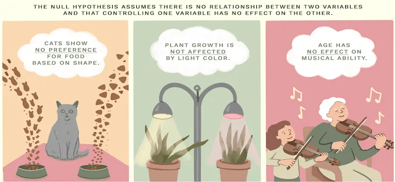
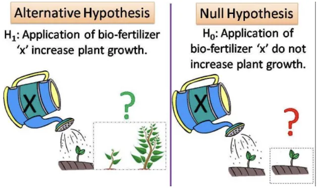
Null Hypothesis (H0)
- A hypothesis of no difference — the default assumption that any observed effect is due to chance alone. Denoted by H0.
- Examples: H0: μ = μ0, H0: μ1 = μ2
Alternative Hypothesis (H1)
- The complement of the null hypothesis — what we believe is true if H0 is rejected. Denoted by H1.
- Examples: H1: μ ≠ μ0, H1: μ1 ≠ μ2
Parameter vs Statistic
| Concept | Belongs To | Symbol | Nature |
|---|---|---|---|
| Parameter | Population | μ, σ² | Fixed but often unknown |
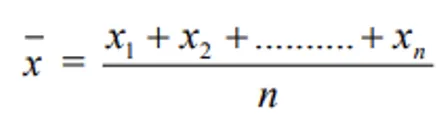
| Statistic | Sample | x̄, s² | Computed from sample data; estimates the parameter |
Different samples yield different statistics — this is precisely why hypothesis testing exists.
Pro Content Locked
Upgrade to Pro to access this lesson and all other premium content.
₹99 charged monthly · Cancel anytime
- All Agriculture & Banking Courses
- AI Lesson Questions (100/day)
- AI Doubt Solver (50/day)
- Glows & Grows Feedback (30/day)
- AI Section Quiz (20/day)
- 22-Language Translation (100/day)
- Recall Questions (20/day)
- AI Quiz (15/day)
- AI Quiz Paper Analysis (100/day)
- AI Step-by-Step Explanations (100/day)
- Spaced Repetition Recall (FSRS)
- AI Tutor
- Immersive Text Questions
- Audio Lessons — Hindi & English
- Mock Tests & Previous Year Papers
- Summary & Mind Maps
- XP, Levels, Leaderboard & Badges
- Generate New Classrooms
- Voice AI Teacher (AgriDots Live)
- AI Revision Assistant
- Knowledge Gap Analysis
- Interactive Revision (LangGraph)
🔒 Secure via Razorpay · Cancel anytime · No hidden fees
A fertiliser company claims its new product increases wheat yield by 20%. An agronomist tests it on 30 plots and finds a 15% increase. Is the difference between the claimed 20% and the observed 15% real, or could it simply be due to natural plot-to-plot variation? Hypothesis testing provides the systematic framework to answer such questions — it is the backbone of statistical inference in agricultural research.
Why Do We Need Hypothesis Testing?
- Sample estimates rarely equal the true population value due to inherent variation.
- Different samples yield different estimates. We must verify whether the difference between a sample estimate and the population value is due to sampling fluctuation or a real difference.
- If the difference is due to sampling fluctuation alone, the sample belongs to the population. If the difference is real, the sample may not belong to that population.
Key Terminology
Hypothesis
- An assumption about any unknown characteristic of a population. It may or may not be true.
- Examples: μ = 2.3, σ = 2.1, or "the population follows Normal Distribution."
- Two types: null hypothesis and alternative hypothesis.
Null Hypothesis (H0)
- A hypothesis of no difference — the default assumption that any observed effect is due to chance alone. Denoted by H0.
- Examples: H0: μ = μ0, H0: μ1 = μ2
Alternative Hypothesis (H1)
- The complement of the null hypothesis — what we believe is true if H0 is rejected. Denoted by H1.
- Examples: H1: μ ≠ μ0, H1: μ1 ≠ μ2
Parameter vs Statistic
| Concept | Belongs To | Symbol | Nature |
|---|---|---|---|
| Parameter | Population | μ, σ² | Fixed but often unknown |
| Statistic | Sample | x̄, s² | Computed from sample data; estimates the parameter |
Different samples yield different statistics — this is precisely why hypothesis testing exists.
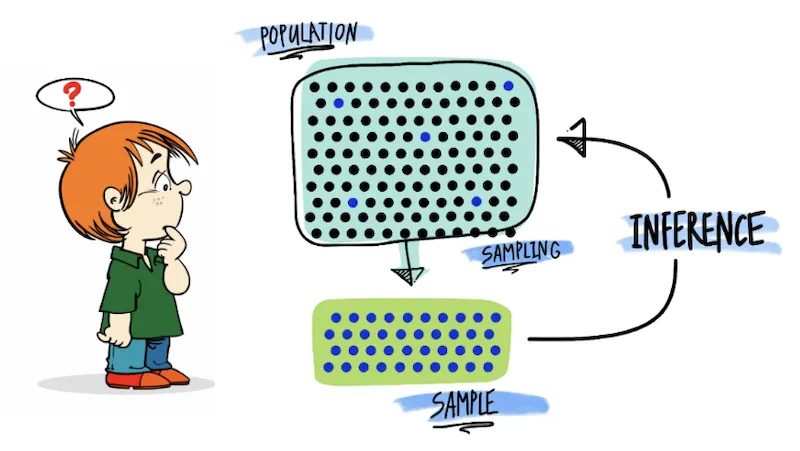
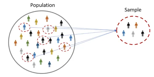
Population and Sample
- Population: The entire group of objects under study — can be finite (students in a class) or infinite (all possible yields of a variety).
- Sample: A finite subset of the population. The number of objects in a sample is the sample size.
Random Sampling (SRS)
- If sampling units are drawn independently with equal chance of inclusion, it is simple random sampling (SRS).
- From a population of N units, the chance of selecting any unit = 1/N.
- Random sampling ensures the sample is representative and eliminates selection bias.
Sampling Distribution and Standard Error
-
Sampling distribution: The distribution of a statistic computed from all possible samples.
-
Standard Error (S.E.): The standard deviation of the sampling distribution.
S.E.(x̄) = σ/√n
-
Increasing sample size n reduces S.E., making the estimate more precise.
Types of Errors
In hypothesis testing, four decisions are possible:
| Type | H0 is true | H0 is false |
|---|---|---|
| Rejecting H0 | Type-I Error (Wrong Decision) | Correct |
| Accepting H0 | Correct | Type-II Error |
| Error | Description | Probability | Analogy | Severity |
|---|---|---|---|---|
| Type I | Rejecting H0 when it is true | Alpha (α) | False alarm — concluding an effect exists when it does not | Controllable |
| Type II | Accepting H0 when it is false | Beta (β) | Missed detection — failing to identify a real effect | More severe |
TIP
Type I = False Positive (seeing an effect that is not there). Type II = False Negative (missing an effect that is there). Type II is considered more severe because genuine improvements go undetected.
Simple vs Composite Hypothesis
| Type | Definition | Example | LOS Expression |
|---|---|---|---|
| Simple | Completely specifies the distribution | H0: μ = μ0, σ known | Exactly α |
| Composite | Does not completely specify distribution | H0: μ ≤ μ0, σ known | At most α |
Degrees of Freedom (d.f.)
- The number of values free to vary in the final calculation of a statistic.
- d.f. = total number of items - total number of constraints = n - k
- Example: If 10 observations have a fixed mean, only 9 are free to vary → d.f. = 10 - 1 = 9.
Level of Significance (LOS)
- The maximum probability of committing Type I Error, denoted by α.
- Common values: 5% (field experiments) and 1%.
- Always fixed in advance before collecting data.
- LOS 5% means results will be correct in 95 out of 100 cases.
IMPORTANT
In agricultural field experiments, 5% LOS is standard — it balances detecting real effects with controlling false positives.
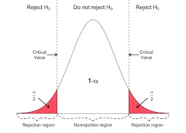
Critical Value
- The threshold that determines whether to reject or accept H0.
- If the test statistic exceeds the critical value, the difference is too large to be explained by chance alone.
Steps in Hypothesis Testing
TIP
Mnemonic: "HSTCR" — Hypothesise, Statistic, Threshold, Compare, Result.
- Formulate the null (H0) and alternative (H1) hypotheses
- Construct the test statistic
- Fix the level of significance
- Find the table (critical) value for the given d.f. and LOS
- Compare calculated value with table value
- Decide:
- If calculated ≥ table value → Reject H0 (significant)
- If calculated < table value → Accept H0 (not significant)
Confidence Limit
- The range within which the true population mean lies is called confidence limit or fiduciary limit.
- A wider interval means less precision but more confidence that the true value is captured.
Summary Table
| Concept | Key Point | Exam Tip |
|---|---|---|
| Null hypothesis (H0) | Hypothesis of no difference | Default assumption to test against |
| Alternative hypothesis (H1) | Complement of H0 | What we conclude if H0 is rejected |
| Parameter | Population characteristic (μ, σ²) | Fixed but unknown |
| Statistic | Sample characteristic (x̄, s²) | Estimate of parameter |
| Type I error (α) | Rejecting true H0 | False positive |
| Type II error (β) | Accepting false H0 | False negative; more severe |
| d.f. | n - k | Free values in calculation |
| LOS | Max probability of Type I error | Usually 5% in agriculture |
| Critical value | Threshold for decision | From statistical tables |
| S.E. | σ/√n | Decreases with larger n |
Summary: Steps in Hypothesis Testing
- Formulate the null (H0) and alternative (H1) hypotheses
- Choose the appropriate test statistic (Z, t, F, or chi-square)
- Fix the level of significance (usually 5%)
- Find the critical (table) value for the given d.f. and LOS
- Compare the calculated value with the table value
- Decide: If calculated > table value, reject H0 (significant). Otherwise, accept H0 (not significant).
Summary Cheat Sheet
| Concept / Topic | Key Details |
|---|---|
| Hypothesis | An assumption about an unknown population characteristic |
| Null hypothesis (H₀) | Hypothesis of no difference — default assumption |
| Alternative hypothesis (H₁) | Complement of H₀; accepted if H₀ is rejected |
| Parameter | Belongs to population (μ, σ²); fixed but unknown |
| Statistic | Belongs to sample (x̄, s²); estimates the parameter |
| Type I error (α) | Rejecting true H₀ — false positive (false alarm) |
| Type II error (β) | Accepting false H₀ — false negative; more severe |
| Degrees of freedom | d.f. = n - k (values free to vary) |
| Level of significance | Max probability of Type I error; usually 5% in agriculture |
| Critical value | Threshold for rejecting or accepting H₀ |
| Standard Error | S.E. = σ/√n; decreases with larger sample size |
| Simple hypothesis | Completely specifies the distribution |
| Composite hypothesis | Does not completely specify the distribution |
| Population | Entire group under study — finite or infinite |
| Sample | Finite subset of population |
| SRS | Simple Random Sampling — each unit has equal chance (1/N) |
| Sampling distribution | Distribution of statistic from all possible samples |
| Confidence limit | Range within which true population mean lies |
| Decision rule | Calc ≥ table value → reject H₀; calc < table → accept H₀ |
| Steps: HSTCR | Hypothesise, Statistic, Threshold, Compare, Result |
| Test types | Z-test (large n), t-test (small n), F-test (variances), χ² (frequencies) |