💃 Probability and Frequency Distributions
Binomial, Poisson, and Normal distributions — properties, transformations, moments, skewness, and kurtosis with agricultural applications
When an entomologist sprays a pesticide on 100 insects, each insect either dies (success) or survives (failure) — a classic two-outcome scenario described by the Binomial distribution. When a plant pathologist counts the rare occurrence of a viral infection across thousands of plants, the Poisson distribution applies. And when an agronomist measures the height of 500 wheat plants, the values cluster symmetrically around an average — the familiar bell curve of the Normal distribution. Understanding these three distributions is essential for choosing the right statistical test in agricultural research.
Probability
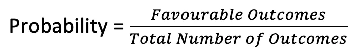
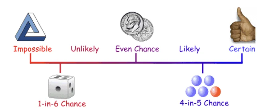
- Range of probability: 0 to 1. A probability of 0 means impossible; 1 means certain.
- Probability of an impossible event = zero.
Types of Distributions
| Type | Variable | Examples |
|---|---|---|
| Discrete | X takes only integer values (0, 1, 2, ...) | Binomial, Poisson |
| Continuous | X takes all possible values in a range | Normal |
Binomial Distribution NABARD 2020 (Mains)
- Given by James Bernoulli in 1700 A.D.
- Models experiments with exactly two possible outcomes: SUCCESS or FAILURE.
Agricultural example: A new pesticide either cures a disease (success, probability p) or does not (failure, probability q).
Pro Content Locked
Upgrade to Pro to access this lesson and all other premium content.
₹99 charged monthly · Cancel anytime
- All Agriculture & Banking Courses
- AI Lesson Questions (100/day)
- AI Doubt Solver (50/day)
- Glows & Grows Feedback (30/day)
- AI Section Quiz (20/day)
- 22-Language Translation (100/day)
- Recall Questions (20/day)
- AI Quiz (15/day)
- AI Quiz Paper Analysis (100/day)
- AI Step-by-Step Explanations (100/day)
- Spaced Repetition Recall (FSRS)
- AI Tutor
- Immersive Text Questions
- Audio Lessons — Hindi & English
- Mock Tests & Previous Year Papers
- Summary & Mind Maps
- XP, Levels, Leaderboard & Badges
- Generate New Classrooms
- Voice AI Teacher (AgriDots Live)
- AI Revision Assistant
- Knowledge Gap Analysis
- Interactive Revision (LangGraph)
🔒 Secure via Razorpay · Cancel anytime · No hidden fees
When an entomologist sprays a pesticide on 100 insects, each insect either dies (success) or survives (failure) — a classic two-outcome scenario described by the Binomial distribution. When a plant pathologist counts the rare occurrence of a viral infection across thousands of plants, the Poisson distribution applies. And when an agronomist measures the height of 500 wheat plants, the values cluster symmetrically around an average — the familiar bell curve of the Normal distribution. Understanding these three distributions is essential for choosing the right statistical test in agricultural research.
Probability
- Range of probability: 0 to 1. A probability of 0 means impossible; 1 means certain.
- Probability of an impossible event = zero.
Types of Distributions
| Type | Variable | Examples |
|---|---|---|
| Discrete | X takes only integer values (0, 1, 2, ...) | Binomial, Poisson |
| Continuous | X takes all possible values in a range | Normal |
Binomial Distribution NABARD 2020 (Mains)
- Given by James Bernoulli in 1700 A.D.
- Models experiments with exactly two possible outcomes: SUCCESS or FAILURE.
Agricultural example: A new pesticide either cures a disease (success, probability p) or does not (failure, probability q).
p + q = 1
Bernoulli Trial
A trial with only two outcomes — success (p) and failure (q) — where each trial is independent of others.
Definition
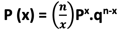
| Parameter | Meaning |
|---|---|
| X | 0, 1, 2, ... (number of successes) |
| n | Number of trials |
| x | Number of successes in n trials |
| p | Probability of success |
| q | Probability of failure (1 - p) |
| Parameters | n and p completely define the distribution |
Three Criteria
- Number of trials is fixed
- Each trial is independent
- Probability of success is constant across trials
Properties
| Property | Value |
|---|---|
| Mean (μ1) | np |
| Variance (μ2) | npq |
| Skewness (μ3) | npq(q - p) |
| Kurtosis (μ4) | npq(1 + 3(n-2)pq) |
| Standard Deviation | √npq |
| Key property | Mean > Variance (since p, q < 1) |
IMPORTANT
In Binomial distribution, the mean is always greater than the variance. This distinguishes it from Poisson (where Mean = Variance).
Poisson Distribution
- Discovered by S.D. Poisson.
- A limiting case of Binomial distribution when n → ∞, p → 0, and np = m (finite).
- Used for independent events occurring at a constant rate within a given interval.
Agricultural examples: Number of diseased plants per field, insect pest counts per trap, defective seeds per batch.
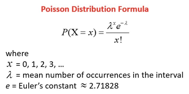
Properties
| Property | Value |
|---|---|
| Mean (μ1) | γ |
| Variance (μ2) | γ |
| μ3 | γ |
| μ4 | 3γ² + γ |
| Key property | Mean = Variance |
IMPORTANT
Mean = Variance is the defining characteristic of Poisson distribution. Use this to test whether data follows Poisson.
- Useful in theory of games, waiting time, business problems.
- Tends to normal distribution when γ → ∞.
Comparison: Binomial vs Poisson
| Feature | Binomial | Poisson |
|---|---|---|
| Discoverer | James Bernoulli | S.D. Poisson |
| Outcomes | Two (success/failure) | Count of rare events |
| Parameters | n and p | m (= np) |
| Mean | np | m |
| Variance | npq | m |
| Mean vs Variance | Mean > Variance | Mean = Variance |
| Agricultural use | Germination success/failure | Pest counts, disease incidence |
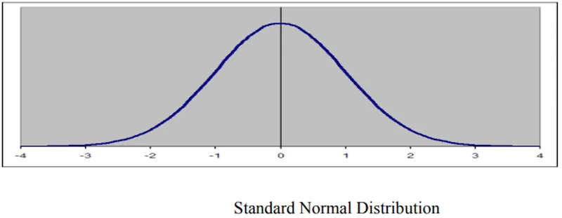
Normal Distribution
- First discovered by De-Moivre in 1733 as the limiting form of the binomial model; independently developed by Laplace and Gauss (hence also called Gaussian distribution).
- Probably the most important distribution in statistics — models both continuous and discrete variables.
- Shape: a bell curve, single mode, symmetric about its central value.
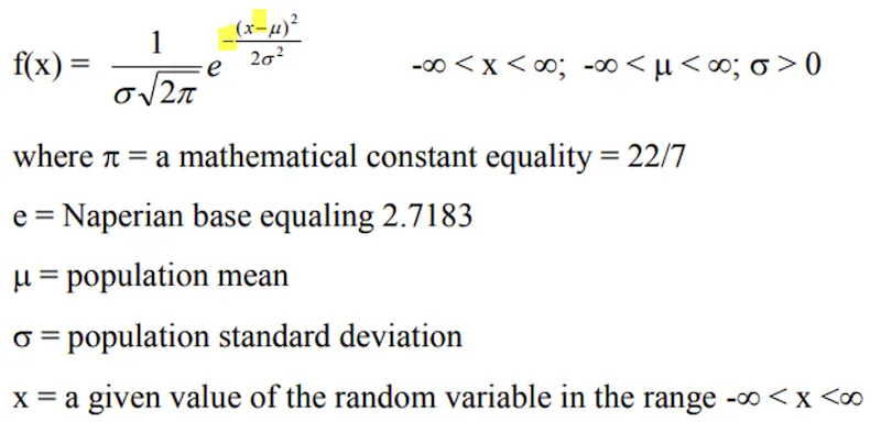
Properties
| Property | Value |
|---|---|
| Central tendency | Mean = Mode = Median |
| Maximum height | At the mean (μ) |
| Skewness (β1) | Zero (perfectly symmetric) |
| Kurtosis (β2) | 3 (Mesokurtic) |
| Odd central moments | All = 0 |
| Quartiles | Q3 - Q2 = Q2 - Q1 |
| Theoretical range | -∞ to +∞ |
| Practical range | 6σ |
| Mean deviation | 4/5 σ |
| Quartile deviation | 2/3 σ |
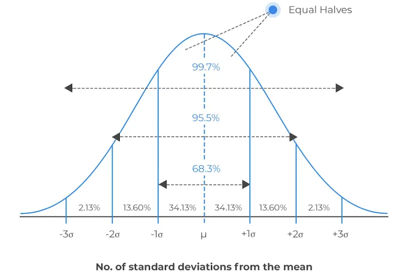
The 68-95-99.7 Rule (Empirical Rule)
| Range | Area Covered |
|---|---|
| μ ± σ | 68.26% |
| μ ± 2σ | 95.44% |
| μ ± 3σ | 99.73% |
IMPORTANT
Memorise the 68-95-99.7 rule — it is frequently tested and extremely useful for quick probability estimates.
Effect of Standard Deviation on Shape
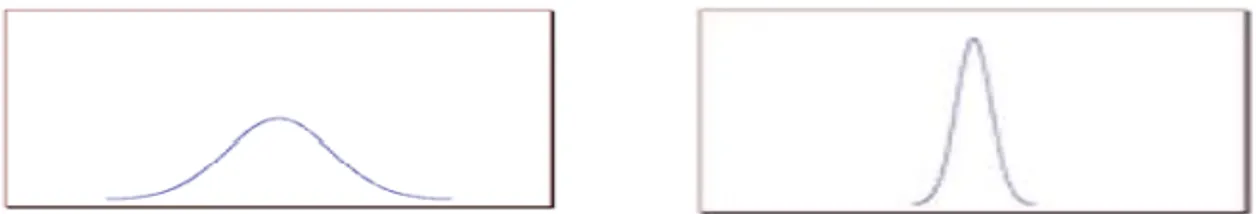
- Large σ → short and wide curve (more spread)
- Small σ → tall and narrow curve (more concentrated)
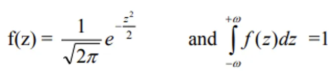
Standard Normal Distribution (SND)
- If X is normal with mean μ and S.D. σ, then Z = (X - μ)/σ is a standard normal variate with mean = 0 and S.D. = 1.
- This standardisation converts any normal distribution into a universal form.
Data Transformation
When data do not follow the normal distribution, we transform the variable to restore normality. This is essential because many tests (ANOVA, t-test) assume normality.
TIP
Mnemonic: "SLA" — Square root for Small counts (Poisson), Log for Large values, Angular for percentage/Binomial data.
| Transformation | When to Use | Formula | Data Type |
|---|---|---|---|
| Square root | Small counts (0-10); Poisson data; percentages > 80% | √x | Count data |
| Logarithmic | Large values with high variation | log x or log(x+1) | Large counts |
| Angular (Arcsine) | Percentages from counts; Binomial data | sinθ = √(p/100) | Percentage data |
Moments
Statistical moments describe frequency distribution characteristics:
| Moment | Measures | Interpretation |
|---|---|---|
| μ1 | Central tendency | Location of the distribution |
| μ2 | Variance | Spread/dispersion |
| μ3 | Skewness | Asymmetry |
| μ4 | Kurtosis | Peakedness/flatness |
- In a symmetric distribution, all odd moments (μ1, μ3, μ5...) = 0.
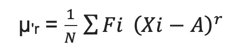
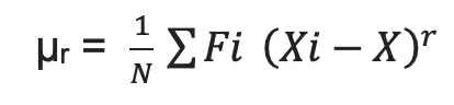
Raw vs Central Moments
| Raw Moment or arbitrary mean | Central moment or Central mean |
|---|---|
| It is denoted by μ'r | It is denoted by μr |
| Calculated about any point | Calculated about mean only and take more time. |
| 1st row moment about point A = 0 is equal to mean. | 1st central moment always zero |
| Raw moment will be changed of origin. | Central moment aren't changed of origin. |
- Raw moment (about arbitrary mean A):
- Central moment (about mean x̄):
| Central Moment | Value | Meaning |
|---|---|---|
| 0th | Always 1 | 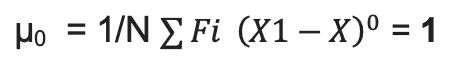 |
| 1st | Always 0 (deviations from mean sum to zero) |  |
| 2nd | Variance |  |
| 3rd | Skewness |  |
| 4th | Kurtosis |  |
Skewness
Symmetric vs Asymmetric Distributions
| Feature | Symmetric | Asymmetric |
|---|---|---|
| Central tendency | Mean = Median = Mode | Mean ≠ Median ≠ Mode |
| Quartiles | Equidistant from median | Not equidistant |
| Curve | Balanced on both sides | Inclined to one side |
| β1 | 0 | ≠ 0 |
Types of Skewness
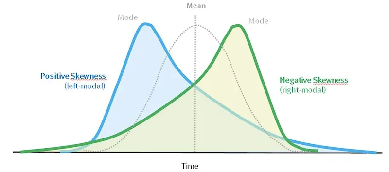
| Type | Tail Direction | Relationship | Agricultural Example |
|---|---|---|---|
| Positive | Longer right tail | Mean > Median > Mode | Farm sizes (many small, few very large) |
| Negative | Longer left tail | Mode > Median > Mean | Maturity period (most late, few very early) |
Measures of Skewness
- Karl Pearson's coefficient:
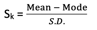
- Based on moments: Skewness (β1) = μ3²/μ2³
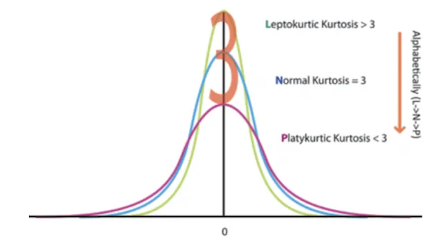
Kurtosis
- Measures the degree of flatness or peakedness of the frequency curve compared to normal distribution.
- Denoted as β2.
| Type | β2 | Shape | Description |
|---|---|---|---|
| Leptokurtic | > 3 | Narrow peak, heavy tails | More concentrated near mean and in tails |
| Mesokurtic | = 3 | Normal curve | Baseline (normal distribution) |
| Platykurtic | < 3 | Flat peak, broad base | More uniformly spread out |
TIP
Mnemonic: Lepto = Lean and tall (peaked), Meso = Medium (normal), Platy = Flat (like a plateau/plate).
Summary Table
| Concept | Key Point | Exam Tip |
|---|---|---|
| Binomial distribution | Two outcomes; Mean > Variance | Given by James Bernoulli |
| Poisson distribution | Rare events; Mean = Variance | Given by S.D. Poisson |
| Normal distribution | Bell curve; Mean = Median = Mode | Given by De-Moivre (1733) |
| 68-95-99.7 rule | Areas under normal curve | Memorise all three percentages |
| Standard Normal | Z = (X-μ)/σ; mean=0, SD=1 | Used for probability tables |
| Square root transform | Poisson data, small counts | √x |
| Log transform | Large values | log x or log(x+1) |
| Angular transform | Percentage/Binomial data | sinθ = √(p/100) |
| Skewness | Departure from symmetry | Positive: Mean > Median > Mode |
| Kurtosis | Peakedness | Lepto > 3, Meso = 3, Platy < 3 |
Summary Cheat Sheet
| Concept / Topic | Key Details |
|---|---|
| Probability range | 0 to 1; impossible event = 0, certain event = 1 |
| Binomial distribution | Given by James Bernoulli (1700 AD); two outcomes only |
| Binomial parameters | n (trials) and p (success probability); Mean = np, Variance = npq |
| Binomial key property | Mean > Variance (distinguishes from Poisson) |
| Poisson distribution | Given by S.D. Poisson; models rare events at constant rate |
| Poisson key property | Mean = Variance |
| Normal distribution | Discovered by De-Moivre (1733); also called Gaussian distribution |
| Normal curve shape | Bell curve, symmetric; Mean = Median = Mode |
| Skewness (Normal) | Zero (perfectly symmetric); Kurtosis β₂ = 3 (Mesokurtic) |
| 68-95-99.7 rule | μ ± 1σ = 68.26%, μ ± 2σ = 95.44%, μ ± 3σ = 99.73% |
| Practical range of Normal | 6σ; Mean deviation = 4/5 σ; Quartile deviation = 2/3 σ |
| Standard Normal Variate | Z = (X - μ)/σ; mean = 0, S.D. = 1 |
| Square root transformation | For Poisson data / small counts (0-10) / percentages > 80% |
| Logarithmic transformation | For large values with high variation; log x or log(x+1) |
| Angular transformation | For percentage/Binomial data; sinθ = √(p/100) |
| Moments | μ₁ = central tendency, μ₂ = variance, μ₃ = skewness, μ₄ = kurtosis |
| Symmetric distribution | All odd moments = 0 |
| Positive skewness | Longer right tail; Mean > Median > Mode |
| Negative skewness | Longer left tail; Mode > Median > Mean |
| Leptokurtic | β₂ > 3 — narrow peak, heavy tails |
| Mesokurtic | β₂ = 3 — normal curve (baseline) |
| Platykurtic | β₂ < 3 — flat peak, broad base |
| Discrete distributions | Binomial and Poisson (integer values) |
| Continuous distribution | Normal (any value in a range) |
| Karl Pearson's skewness | (Mean - Mode) / S.D. |