👐🏻 Measures of Dispersion
Range, Quartile Deviation, Mean Deviation, Standard Deviation, Variance, Coefficient of Variation, and Standard Error — with agricultural examples
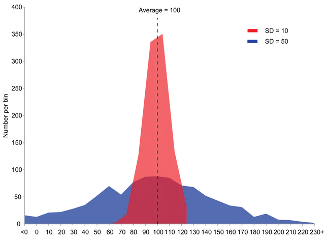
Consider two groundnut varieties, both yielding an average of 50 kg per plot. Should a farmer be indifferent between them? Not at all — if the first variety consistently yields 48-52 kg while the second swings between 20-80 kg, the first is clearly more reliable. This is why we need measures of dispersion: the mean alone never tells the full story.
What Is Dispersion?
- Dispersion means scattering of observations among themselves or from a central value (Mean/Median/Mode). While central tendency gives the "typical" value, dispersion tells us how spread out the data is around that value.
Agricultural Example
| Variety 1 | 46 | 48 | 50 | 52 | 54 |
| Variety 2 | 30 | 40 | 50 | 60 | 70 |
- Both varieties have a mean yield of 50 kg, yet Variety 1 is more consistent (uniform) and Variety 2 shows more variability. A farmer would prefer Variety 1 for its reliability.
Types of Measures
| Type | Nature | Unit | Use |
|---|---|---|---|
| Absolute measures | Actual spread | Same as data | Describe dispersion in original units |
| Relative measures | Ratio/coefficient | Unit-free | Compare dispersion across different datasets |
Absolute Measures
1. Range
- The simplest measure of dispersion — considers only the two extreme values.
Range = Largest value - Smallest value Coefficient of range = (L - S)/(L + S)
Pro Content Locked
Upgrade to Pro to access this lesson and all other premium content.
₹99 charged monthly · Cancel anytime
- All Agriculture & Banking Courses
- AI Lesson Questions (100/day)
- AI Doubt Solver (50/day)
- Glows & Grows Feedback (30/day)
- AI Section Quiz (20/day)
- 22-Language Translation (100/day)
- Recall Questions (20/day)
- AI Quiz (15/day)
- AI Quiz Paper Analysis (100/day)
- AI Step-by-Step Explanations (100/day)
- Spaced Repetition Recall (FSRS)
- AI Tutor
- Immersive Text Questions
- Audio Lessons — Hindi & English
- Mock Tests & Previous Year Papers
- Summary & Mind Maps
- XP, Levels, Leaderboard & Badges
- Generate New Classrooms
- Voice AI Teacher (AgriDots Live)
- AI Revision Assistant
- Knowledge Gap Analysis
- Interactive Revision (LangGraph)
🔒 Secure via Razorpay · Cancel anytime · No hidden fees
Consider two groundnut varieties, both yielding an average of 50 kg per plot. Should a farmer be indifferent between them? Not at all — if the first variety consistently yields 48-52 kg while the second swings between 20-80 kg, the first is clearly more reliable. This is why we need measures of dispersion: the mean alone never tells the full story.
What Is Dispersion?
- Dispersion means scattering of observations among themselves or from a central value (Mean/Median/Mode). While central tendency gives the "typical" value, dispersion tells us how spread out the data is around that value.
Agricultural Example
| Variety 1 | 46 | 48 | 50 | 52 | 54 |
| Variety 2 | 30 | 40 | 50 | 60 | 70 |
- Both varieties have a mean yield of 50 kg, yet Variety 1 is more consistent (uniform) and Variety 2 shows more variability. A farmer would prefer Variety 1 for its reliability.
Types of Measures
| Type | Nature | Unit | Use |
|---|---|---|---|
| Absolute measures | Actual spread | Same as data | Describe dispersion in original units |
| Relative measures | Ratio/coefficient | Unit-free | Compare dispersion across different datasets |
Absolute Measures
1. Range
- The simplest measure of dispersion — considers only the two extreme values.
Range = Largest value - Smallest value Coefficient of range = (L - S)/(L + S)
- In industries for quality control, the most important measure of dispersion is Range. Quick to compute, gives an immediate sense of spread.
2. Quartile Deviation
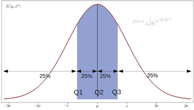
- Quartile Deviation (Semi-Interquartile Range) = (Q3 - Q1)/2
- Quartile Range = Q3 - Q1
- Coefficient of quartile range = (Q3 - Q1)/(Q3 + Q1)
Measures the spread of the middle 50% of data — more resistant to outliers than range because it ignores the extreme 25% on each side.
3. Mean Deviation
- For ungrouped data: M.D. = ∑|Xi - X|/N
- For grouped data: M.D. = ∑f|Xi - X|/N
Measures the average of absolute deviations from the mean (or median). Uses absolute values to prevent positive and negative deviations from cancelling out. However, it is not as mathematically convenient as standard deviation for further analysis.
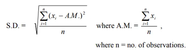
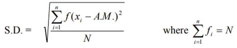
4. Standard Deviation (S.D.)

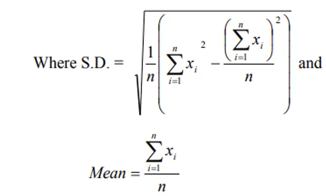
- The positive square root of the arithmetic mean of the squares of deviations from the arithmetic mean.
- The square of S.D. is called variance.
S.D. = √Variance
- Given by Karl Pearson (1823), denoted by Greek letter sigma (σ).
IMPORTANT
Standard Deviation is the best measure of dispersion — least affected by sampling fluctuations, uses all observations, and is used in nearly all advanced statistical procedures.
| Property | Value |
|---|---|
| Range of S.D. | 0 to ∞ |
| S.D. = 0 means | No variation — all observations identical |
| Negative values | S.D. is always positive (due to squaring) |
| Sampling stability | Least affected by sampling fluctuations |
Ungrouped Data Formulas
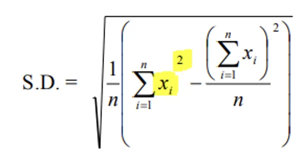
By linear transformation:
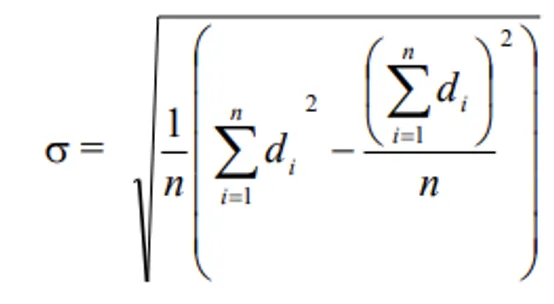
Where di = xi - A, A = Assumed value.
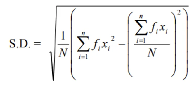
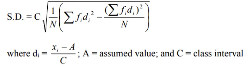
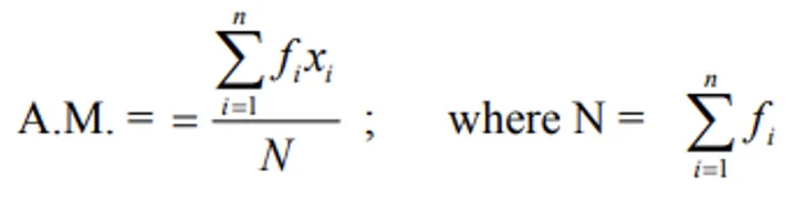
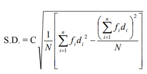
Grouped Data Formulas
By linear transformation:
Examples
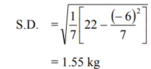
Ungrouped: Kapas yields (kg/plot) of cotton from 7 plots: 5, 6, 7, 7, 9, 4, 5
| xi | xi2 | di = xi - A | di2 |
|---|---|---|---|
| 5 | 25 | 5-7 = -2 | 4 |
| 6 | 36 | 6-7 = -1 | 1 |
| 7 | 49 | 7-7 = 0 | 0 |
| 7 | 49 | 7-7 = 0 | 0 |
| 9 | 81 | 9-7 = 2 | 4 |
| 4 | 16 | 4-7 = -3 | 9 |
| 5 | 25 | 5-7 = -2 | 4 |
| ∑xi = 43 | ∑xi2 = 281 | ∑di = -6 | ∑di2 = 22 |
Direct method:
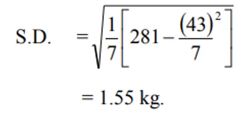
Deviation method:
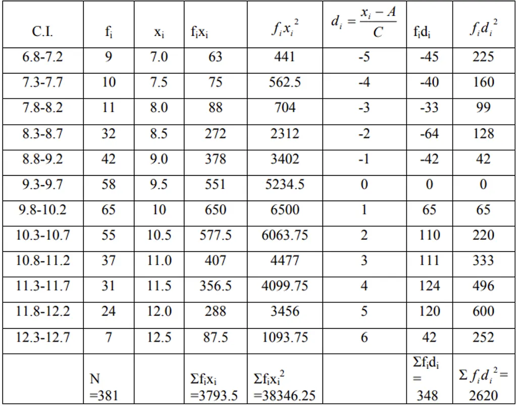
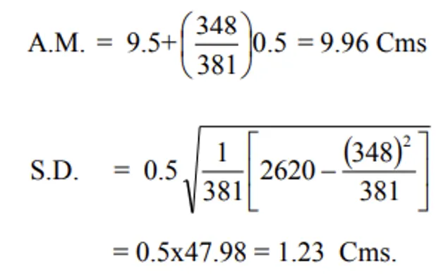
Grouped: 381 soybean plant heights (cm):
| Plant heights (Cms) | No. of Plants (fi) |
|---|---|
| 6.8-7.2 | 9 |
| 7.3-7.7 | 10 |
| 7.8-8.2 | 11 |
| 8.3-8.7 | 32 |
| 8.8-9.2 | 42 |
| 9.3-9.7 | 58 |
| 9.8-10.2 | 65 |
| 10.3-10.7 | 55 |
| 10.8-11.2 | 37 |
| 11.3-11.7 | 31 |
| 11.8-12.2 | 24 |
| 12.3-12.7 | 7 |
i) Direct method:
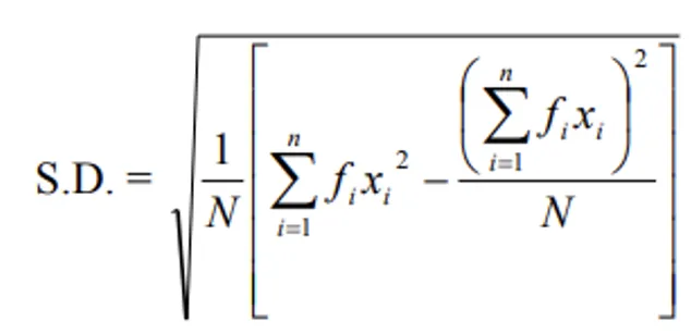
ii) Deviation method:
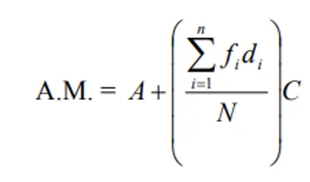
i) Direct method:
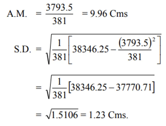
ii) Deviation method:
Variance
- Term variance proposed by R.A. Fisher.
- Square of standard deviation is variance.
- Expressed in squared units — plays a crucial role in ANOVA, regression analysis, and many other procedures.
Relative Measures of Dispersion
When comparing two datasets with different units or different means, absolute measures are inadequate. We need relative measures — unit-free ratios called coefficients.
Coefficient of Variation (C.V.)
- Given by Karl Pearson.
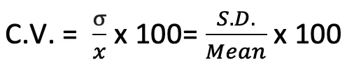
- C.V. = (S.D./Mean) x 100
- Greater C.V. = more variability (less homogeneity); lower C.V. = more consistency.
- Unit-less measure — can compare variability between datasets with completely different units.
NOTE
Standard deviation is an absolute measure; C.V. is a relative measure. Use C.V. when comparing datasets with different units or means.
Example
Two groundnut varieties:
- Variety 1: Mean = 82 kg, S.D. = 16 kg
- Variety 2: Mean = 55 kg, S.D. = 8 kg
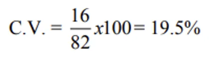
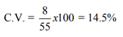
Variety 2 has lower C.V. — less variability despite having a lower S.D. in absolute terms. This perfectly illustrates why C.V. is preferred over S.D. when means differ.
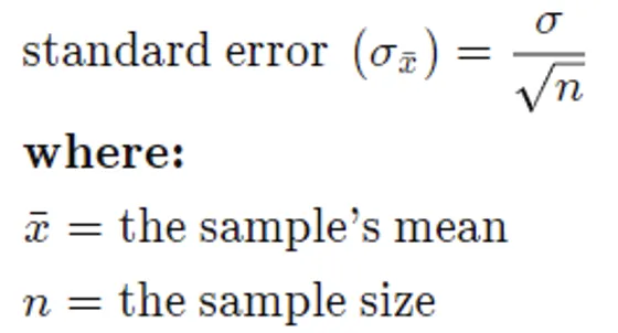
Standard Error of Mean (SEM)
- S.D. of the sampling distribution of means — tells us how much the sample mean is expected to fluctuate from sample to sample.
| Property | Detail |
|---|---|
| SEM vs S.D. | SEM is always smaller than S.D. |
| Purpose | Measures precision of sample mean |
| For higher precision | Use larger samples (as n increases, SEM decreases) |
Comparison of All Measures
| Measure | Type | Formula | Key Feature | Agricultural Use |
|---|---|---|---|---|
| Range | Absolute | L - S | Simplest; only extremes | Quality control in industries |
| Quartile Deviation | Absolute | (Q3-Q1)/2 | Resistant to outliers | Describing middle 50% of yield data |
| Mean Deviation | Absolute | ∑|x-mean|/n | Uses all observations | Less common; easier to understand |
| Standard Deviation | Absolute | √(∑(x-mean)²/n) | Best measure; least sampling effect | ANOVA, regression, all advanced analysis |
| Variance | Absolute | S.D.² | Squared units | Fisher's ANOVA, F-test |
| C.V. | Relative | (S.D./Mean)x100 | Unit-free | Comparing variability across crops/varieties |
| SEM | Relative | S.D./√n | Precision of mean estimate | Reporting treatment means in experiments |
TIP
Exam mnemonic for best measures:
- Best measure of central tendency = Arithmetic Mean
- Best measure of dispersion = Standard Deviation
- Best relative measure = Coefficient of Variation
- All three were championed by Karl Pearson and R.A. Fisher.
Summary Cheat Sheet
| Concept / Topic | Key Details |
|---|---|
| Dispersion | Scattering of observations from a central value |
| Absolute measures | Same unit as data — Range, Q.D., M.D., S.D., Variance |
| Relative measures | Unit-free ratios — C.V., SEM |
| Range | Largest - Smallest; simplest measure; used in quality control |
| Quartile Deviation | (Q₃ - Q₁)/2; measures spread of middle 50% |
| Mean Deviation | Average of absolute deviations from mean |
| Standard Deviation | Given by Karl Pearson (1823); denoted by σ |
| S.D. = best measure | Least affected by sampling fluctuations; uses all observations |
| S.D. range | 0 to ∞; S.D. = 0 means no variation (all values identical) |
| Variance | Square of S.D.; term coined by R.A. Fisher |
| Variance units | Squared units of original data |
| Coefficient of Variation | C.V. = (S.D./Mean) x 100; given by Karl Pearson |
| C.V. interpretation | Greater C.V. = more variability; lower C.V. = more consistent |
| C.V. advantage | Unit-less — can compare datasets with different units/means |
| Standard Error (SEM) | S.D. of sampling distribution of means = σ/√n |
| SEM vs S.D. | SEM is always smaller than S.D. |
| Higher precision | Use larger samples (as n increases, SEM decreases) |
| Best central tendency | Arithmetic Mean |
| Best dispersion measure | Standard Deviation |
| Best relative measure | Coefficient of Variation |
| Ungrouped S.D. formula | √(∑(x - mean)²/n) or by linear transformation method |
| Grouped S.D. | Uses mid-values and frequencies with deviation method |
| Consistency comparison | Variety with lower C.V. is more consistent |
| SEM purpose | Measures precision of sample mean estimate |