👨👧👧 Measures of Central Tendency
Arithmetic Mean, Median, Mode, Geometric Mean, Harmonic Mean — formulas, properties, merits, demerits, and agricultural examples
A plant breeder weighs 100 sorghum ear-heads and records values ranging from 60 g to 140 g. To communicate these results in a single number — "the typical ear-head weight" — she needs a measure of central tendency. But which one should she use? The answer depends on the data's nature and distribution.
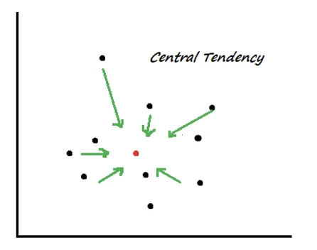
What Is Central Tendency?
- Any mathematical measure intended to represent the center or central value of a set of observations is a measure of central tendency (also called a measure of location or an average).
- It answers the question: "What is the typical or representative value of this dataset?"
Characteristics of a Satisfactory Average
TIP
Exam mnemonic: REBALL — Rigidly defined, Easy to calculate, Based on all observations, Algebraic treatment possible, Least affected by sampling, Located easily.
- Rigidly defined — no ambiguity in computation
- Easy to understand and calculate
- Based on all the observations
- Least affected by sampling fluctuations
- Capable of further algebraic treatment
- Not much affected by extreme values
- Easily located
Overview of All Measures
| Measure | Best Used For | Formula Basis | Key Property |
|---|---|---|---|
| Arithmetic Mean | General average | Sum / Count | Least affected by sampling fluctuations |
| Median | Skewed data, qualitative ranking | Middle value | Not affected by extreme values |
| Mode | Most common value, business forecasting | Maximum frequency | Easy to find by inspection |
| Geometric Mean | Growth rates, bacterial counts | n-th root of product | Zero if any value is zero |
| Harmonic Mean | Speeds, rates, ratios | Reciprocal of mean of reciprocals | Gives more weight to smaller values |
Arithmetic Mean (A.M.)
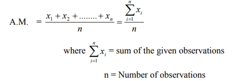
- The sum of observations divided by the number of observations — the most commonly used and widely understood measure.
- A.M. is measured in the same units as the observations.
Ungrouped Data — Direct Method
Let x1, x2, ..., xn be 'n' observations:
Pro Content Locked
Upgrade to Pro to access this lesson and all other premium content.
₹99 charged monthly · Cancel anytime
- All Agriculture & Banking Courses
- AI Lesson Questions (100/day)
- AI Doubt Solver (50/day)
- Glows & Grows Feedback (30/day)
- AI Section Quiz (20/day)
- 22-Language Translation (100/day)
- Recall Questions (20/day)
- AI Quiz (15/day)
- AI Quiz Paper Analysis (100/day)
- AI Step-by-Step Explanations (100/day)
- Spaced Repetition Recall (FSRS)
- AI Tutor
- Immersive Text Questions
- Audio Lessons — Hindi & English
- Mock Tests & Previous Year Papers
- Summary & Mind Maps
- XP, Levels, Leaderboard & Badges
- Generate New Classrooms
- Voice AI Teacher (AgriDots Live)
- AI Revision Assistant
- Knowledge Gap Analysis
- Interactive Revision (LangGraph)
🔒 Secure via Razorpay · Cancel anytime · No hidden fees
A plant breeder weighs 100 sorghum ear-heads and records values ranging from 60 g to 140 g. To communicate these results in a single number — "the typical ear-head weight" — she needs a measure of central tendency. But which one should she use? The answer depends on the data's nature and distribution.
What Is Central Tendency?
- Any mathematical measure intended to represent the center or central value of a set of observations is a measure of central tendency (also called a measure of location or an average).
- It answers the question: "What is the typical or representative value of this dataset?"
Characteristics of a Satisfactory Average
TIP
Exam mnemonic: REBALL — Rigidly defined, Easy to calculate, Based on all observations, Algebraic treatment possible, Least affected by sampling, Located easily.
- Rigidly defined — no ambiguity in computation
- Easy to understand and calculate
- Based on all the observations
- Least affected by sampling fluctuations
- Capable of further algebraic treatment
- Not much affected by extreme values
- Easily located
Overview of All Measures
| Measure | Best Used For | Formula Basis | Key Property |
|---|---|---|---|
| Arithmetic Mean | General average | Sum / Count | Least affected by sampling fluctuations |
| Median | Skewed data, qualitative ranking | Middle value | Not affected by extreme values |
| Mode | Most common value, business forecasting | Maximum frequency | Easy to find by inspection |
| Geometric Mean | Growth rates, bacterial counts | n-th root of product | Zero if any value is zero |
| Harmonic Mean | Speeds, rates, ratios | Reciprocal of mean of reciprocals | Gives more weight to smaller values |
Arithmetic Mean (A.M.)
- The sum of observations divided by the number of observations — the most commonly used and widely understood measure.
- A.M. is measured in the same units as the observations.
Ungrouped Data — Direct Method
Let x1, x2, ..., xn be 'n' observations:
Ungrouped Data — Deviation Method
When observations are large, the Linear Transformation Method simplifies calculation:
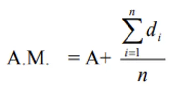
Where:
- A = Assumed mean (usually the mid-point of the middle class or the class with highest frequency)
- di = xi - A
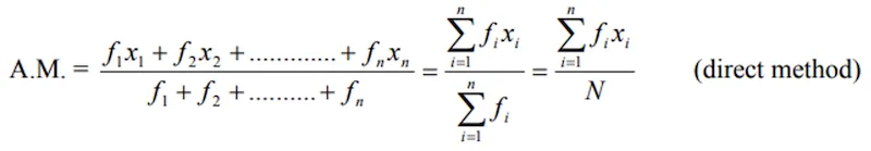
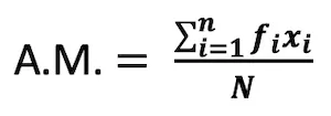
Grouped Data
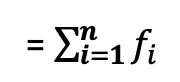
Let f1, f2, ..., fn be frequencies corresponding to mid-values x1, x2, ..., xn:
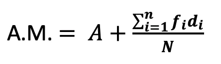
By deviation method:
Where di = (xi - A)/C, f = frequency, C = class interval, x = mid-values.
- Population mean is denoted by μ; sample mean by X (an estimate of μ). This distinction is fundamental in statistics.
Properties of A.M.
-
The algebraic sum of deviations from the arithmetic mean is zero:
∑(x - A.M.) = 0
-
Combined mean (weighted mean) of k groups:
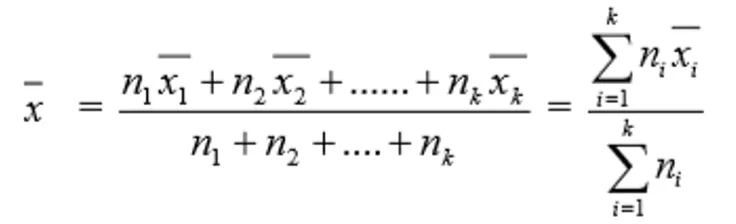
Sampling Fluctuation: The variation in sample statistics from sample to sample. For example, different random samples of 5 plants from a population of 30 will yield different sample means.
Merits and Demerits
| Merits | Demerits |
|---|---|
| Rigidly defined by formula | Cannot be determined by inspection or graphically |
| Most commonly used, best of all averages | Cannot be computed if a single observation is missing |
| Least affected by sampling fluctuations | Heavily affected by extreme values |
| Based on all observations | Misleading for extremely skewed distributions |
| Amenable to further algebraic treatment | |
| Best for finding average height of plants |
Examples
i) Ungrouped data: Weights of 7 sorghum ear-heads: 89, 94, 102, 107, 108, 115, 126 g.
| xi | di = xi - A |
|---|---|
| 89 | 89 - 102 = -13 |
| 94 | 94 - 102 = -8 |
| 102 | 102 - 102 = 0 |
| 107 | 107 - 102 = 5 |
| 108 | 108 - 102 = 6 |
| 115 | 115 - 102 = 13 |
| 126 | 126 - 102 = 24 |
| ∑x = 741 | ∑d = 29 |
- A = 102, AM = 741/7 = 105.86 g
- By deviation method: AM = 102 + (27/7) = 105.86 g
ii) Grouped Data: 405 soybean plant heights from a plot:
| Plant height (cm) | 8-12 | 13-17 | 18-22 | 23-27 | 28-32 | 33-37 | 38-42 | 43-47 | 48-52 | 53-57 |
|---|---|---|---|---|---|---|---|---|---|---|
| No. of plants (fi) | 6 | 17 | 25 | 86 | 125 | 77 | 55 | 9 | 4 | 1 |
a) Direct Method:
b) Deviation Method: (C = 5, A = 30)
- Direct Method: A.M. = 12270/405 = 30.30 cm
- Deviation Method: A.M. = 30 + (24/405) x 5 = 30.30 cm
Median
- The value of the middle-most item when data is arranged in ascending or descending order. It divides the dataset into two equal halves — 50% below, 50% above.
- Used for qualitative data such as intelligence, ability, and honesty. Especially useful for skewed distributions where the mean may be misleading.
NOTE
Unlike the arithmetic mean, the median is not affected by extreme values (outliers), making it robust for skewed data.
Ungrouped Data
- Odd n: Median = the middle value after arrangement.
- Even n: Median = arithmetic mean of the two middle terms.
- Formula: Median = Size of (N+1)/2, where N = ∑f
Continuous Frequency Distribution
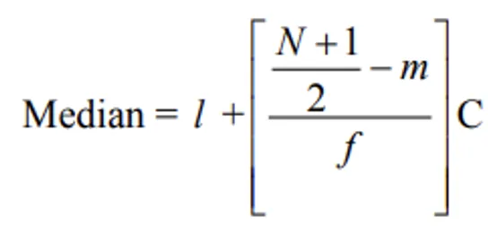
Where: l = lower limit of median class, f = frequency of median class, m = cumulative frequency of preceding class, C = class length, N = total frequency.
Examples
Case i) Odd n: Runs scored by 11 players: 5, 19, 42, 11, 50, 30, 21, 0, 52, 36, 27
- Arranged: 0, 5, 11, 19, 21, 27, 30, 36, 42, 50, 52
- Median = 6th value = 27 runs
Case ii) Even n: Plant heights: 6, 10, 4, 3, 9, 11, 22, 18
- Arranged: 3, 4, 6, 9, 10, 11, 18, 22
- Median = Average of 4th and 5th = (9 + 10)/2 = 9.5 cm
Grouped Data: 180 sorghum ear-heads:
| Weight of ear-heads (in g) | No. of ear-heads | Cumulative Frequency (CF) |
|---|---|---|
| 40-60 | 6 | 6 |
| 60-80 | 28 | 34 |
| 80-100 | 35 | 69 - m |
| 100-120 | 45 - f | 114 (Median class) |
| 120-140 | 30 | 144 |
| 140-160 | 15 | 159 |
| 160-180 | 12 | 171 |
| 180-200 | 9 | 180 |
| N = ∑f = 180 |
- Median class = 100-120, Median = 100 + ((90.5-69)/45) x 20 = 109.56 g
Merits and Demerits
| Merits | Demerits |
|---|---|
| Rigidly defined | Not exact for even n (estimated) |
| Easy to understand; can be located by inspection | Not amenable to algebraic treatment |
| Not affected by extreme values | More affected by sampling fluctuations than mean |
| Works with open-end classes |
Mode
- The value occurring most frequently in a dataset — the most common or most popular value.
- Example: 4, 7, 6, 5, 4, 6, 4 → Mode = 4
- Used for: model size of shoes, readymade garments, business/meteorological forecasting
Continuous Frequency Distribution
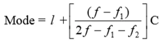
Where: l = lower limit of modal class, C = class interval, f = frequency of modal class, f1 and f2 = frequencies of preceding and succeeding classes.
Examples
Ungrouped: 27, 28, 30, 33, 31, 35, 34, 33, 40, 41, 55, 46, 31, 33, 36, 33, 41, 33 → Mode = 33 (appears 5 times)
Grouped: Marks of 89 students:
| Marks | 10-14 | 15-19 | 20-24 | 25-29 | 30-34 | 35-39 | 40-44 | 45-49 |
|---|---|---|---|---|---|---|---|---|
| No. of students | 4 | 6 | 10 | 16 | 21 | 18 | 9 | 5 |
| Marks | No. of students (f) |
|---|---|
| 10-14 | 4 |
| 15-19 | 6 |
| 20-24 | 10 |
| 25-29 | 16f1 |
| 30-34 | 21f |
| 35-39 | 18f2 |
| 40-44 | 9 |
| 45-49 | 5 |
- Modal class = 29.5-34.5, Mode = 30 + [(21-16)/(2x21-16-18)] x 5 = 33.63
Merits and Demerits
| Merits | Demerits |
|---|---|
| Easy to calculate and comprehend | Ill-defined; may have two modes (bimodal) or more (multimodal) |
| Not affected by extreme values | Not based on all observations |
| Works with unequal class intervals and open-end classes | Not capable of further mathematical treatment |
| More affected by sampling fluctuations than mean |
Harmonic Mean
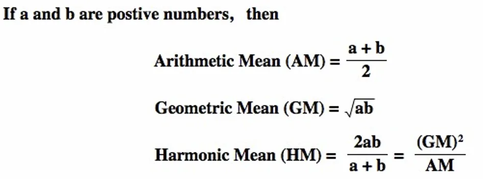
- The reciprocal of the arithmetic average of the reciprocals of given values. Gives more weight to smaller values.
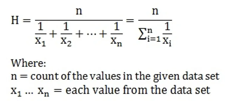
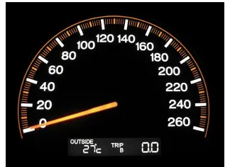
- Used to find average speed, distance, and rate. For example, if you travel equal distances at different speeds, the harmonic mean gives the correct average speed.
Geometric Mean
- The nth root of the product of n observations. Appropriate for data that is multiplicative or involves growth rates.
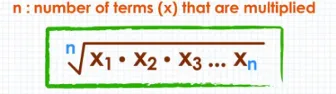
- If any observation is zero, G.M. = zero.
- Used in: bacterial growth, cell division, and wherever values grow by multiplication.
Key Relationships
IMPORTANT
These relationships are high-frequency exam questions. Memorise them!
| Relationship | Formula |
|---|---|
| Symmetrical distribution | Mean = Mode = Median |
| Skewed distribution (empirical) | Mode = 3 Median - 2 Mean |
| AM, GM, HM inequality | AM >= GM >= HM (equal only when all values are identical) |
| GM from AM and HM | G.M. = √(A.M. x H.M.) |
Summary Table
| Measure | Formula | Best For | Key Limitation | Exam Tip |
|---|---|---|---|---|
| A.M. | ∑x/n | General average, plant heights | Affected by outliers | Best and most commonly used |
| Median | Middle value | Skewed data, qualitative ranking | Not algebraically tractable | Not affected by extremes |
| Mode | Most frequent value | Shoe sizes, forecasting | May not be unique | Can be located by inspection |
| G.M. | (x1.x2...xn)1/n | Growth rates, bacteria | Zero if any value is zero | Used in cell division studies |
| H.M. | n/∑(1/x) | Speeds, rates | Undefined if any value is zero | Correct average for equal-distance travel |
TIP
Mnemonic for the AM-GM-HM inequality: "All Grapes Have" decreasing sizes — AM is always largest, GM in the middle, HM smallest.
Explore More 🔭
🟢 Central Tendency — Video Explanation
Summary Cheat Sheet
| Concept / Topic | Key Details |
|---|---|
| Central tendency | A single value representing the center of a dataset |
| Arithmetic Mean (A.M.) | Sum of observations / number of observations; most commonly used |
| A.M. key property | Sum of deviations from mean = zero; least affected by sampling fluctuations |
| A.M. limitation | Heavily affected by extreme values (outliers) |
| Population mean symbol | μ; Sample mean symbol = X̄ |
| Median | Middle-most value in ordered data; divides data into two equal halves |
| Median strength | Not affected by extreme values; works with open-end classes |
| Mode | Value occurring most frequently; located by inspection |
| Mode limitation | May be bimodal or multimodal; not based on all observations |
| Geometric Mean (G.M.) | n-th root of product of n observations; used for growth rates, bacterial counts |
| G.M. = 0 if | Any observation is zero |
| Harmonic Mean (H.M.) | Reciprocal of mean of reciprocals; used for average speed/rate |
| AM-GM-HM inequality | AM ≥ GM ≥ HM (equal only when all values identical) |
| G.M. from AM and HM | G.M. = √(AM x HM) |
| Symmetric distribution | Mean = Mode = Median |
| Skewed distribution | Mode = 3 Median - 2 Mean (empirical relation) |
| Best average | Arithmetic Mean — rigidly defined, algebraically tractable |
| Best for skewed data | Median — robust to outliers |
| Best for forecasting | Mode — most popular/common value |
| Best for speeds/rates | Harmonic Mean — correct average for equal-distance travel |
| Best for cell division | Geometric Mean — multiplicative data |
| Combined mean | Weighted mean of k groups using group sizes and means |
| Deviation method | Uses assumed mean (A) to simplify calculation |
| Satisfactory average | Rigidly defined, easy, based on all observations, algebraically tractable |