📊 Split plot design

This lesson builds core statistical understanding for BSc Agriculture exam preparation through clear concepts, worked structures, and application-focused interpretation.

---

Split plot design – layout – ANOVA Table

Split-plot Design

In field experiments certain factors may require larger plots than for others. For example, experiments on irrigation, tillage, etc requires larger areas. On the other hand experiments on fertilizers, etc may not require larger areas. To accommodate factors which require different sizes of experimental plots in the same experiment, split plot design has been evolved. In this design, larger plots are taken for the factor which requires larger plots. Next each of the larger plots is split into smaller plots to accommodate the other factor. The different treatments are allotted at random to their respective plots. Such arrangement is called split plot design. In split plot design the larger plots are called main plots and smaller plots within the larger plots are called as sub plots. The factor levels allotted to the main plots are main plot treatments and the factor levels allotted to sub plots are called as sub plot treatments.

Layout and analysis of variance table

First the main plot treatment and sub plot treatment are usually decided based on the needed precision. The factor for which greater precision is required is assigned to the sub plots. The replication is then divided into number of main plots equivalent to main plot treatments. Each main plot is divided into subplots depending on the number of sub plot treatments. The main plot treatments are allocated at random to the main plots as in the case of RBD. Within each main plot the sub plot treatments are allocated at random as in the case of RBD. Thus randomization is done in two stages. The same procedure is followed for all the replications independently.

The analysis of variance will have two parts, which correspond to the main plots and sub-plots. For the main plot analysis, replication X main plot treatments table is formed. From this two-way table sum of squares for replication, main plot treatments and error (a) are computed. For the analysis of sub-plot treatments, main plot X sub-plot treatments table is formed. From this table the sums of squares for sub-plot treatments and interaction between main plot and sub-plot treatments are computed. Error (b) sum of squares is found out by residual method. The analysis of variance table for a split plot design with m main plot treatments and s sub-plot treatments is given below.

Analysis of variance for split plot with factor A with m levels in main plots and factor B with s levels in sub-plots will be as follows:

Sources of

Variation	d.f.	SS	MS	F
Replication	r-1	RSS	RMS	RMS/EMS (a)
A	m-1	ASS	AMS	AMS/EMS (a)
Error (a)	(r-1) (m-1)	ESS (a)	EMS (a)
B	s-1	BSS	BMS	BMS/EMS (b)
AB	(m-1) (s-1)	ABSS	ABMS	ABMS/EMS (b)
Error (b)	m(r-1) (s-1)	ESS (b)	EMS (b)
Total rms – 1 TSS

Analysis

Arrange the results as follows

Treatment Combination | Replication | Total

---|---|---

R1 | R2 | R3 | …

A0B0 | a0b0 | a0b0 | a0b0 | … | T00 A0B1 | a0b1 | a0b1 | a0b1 | … | T01 A0B2 | a0b2 | a0b2 | a0b2 | … | T02 Sub Total | A01 | A02 | A03 | … | T0 A1B0 | a1b0 | a1b0 | a1b0 | … | T10 A1B1 | a1b1 | a1b1 | a1b1 | … | T11 A1B2 | a1b2 | a1b2 | a1b2 | … | T12 Sub Total | A11 | A12 | A13 | … | T1 . . . | . . . | . . . | . . . | . . . | . . . Total | R1 | R2 | R3 | … | G.T

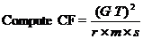
TSS=[ (a0b0)2 + (a0b1)2+(a0b2)2+…]-CF

Form A x R Table and calculate RSS, ASS and Error (a) SS

Treatment	Replication	Total
R1	R2	R3
A0	A01	A02
A1	A11	A12
A2	A21	A22
.
.
.	.
.
.	.
.
.	.
.
.	.
.
.	.
.
.
Total	R1	R2

Error (a) SS= A x R TSS-RASS-ASS. Form A xB Table and calculate BSS, Ax B SSS and Error (b) SS

Treatment	Replication	Total
B0	B1	B2
A0	T00	T01
A1	T10	T11
A2	T20	T21
.
.
.	.
.
.	.
.
.	.
.
.	.
.
.	.
.
.
Total	C0	C1

ABSS= A x B Table SS – ASS- ABSS Error (b) SS= Table SS-ASS-BSS-ABSS –Error (a) SS. Then complete the ANOVA table.

---|---

Summary Cheat Sheet

• Focus: core definitions, classification logic, and design/analysis workflow from this lesson.
• Exam Use: revise key terms, assumptions, and interpretation steps for objective and descriptive questions.
• Practice: solve one representative numerical or conceptual question from this topic.

References

1 source • [1]

[1]

Standard BSc Agriculture Statistics notes used for lesson preparation.