💻 Maxima & Minima of several

This lesson covers core applied mathematics concepts and their agricultural applications for BSc Agriculture learners.

---

MATHS :: Lecture 13 :: Maxima & Minima of several variables

PHYSICAL AND ECONOMIC OPTIMUM FOR SINGLE INPUT Let y = f(x) be a response function. Here x stands for the input that is kgs of fertilizer applied per hectare and y the corresponding output that is kgs of yield per hectare. We know that the maximum is only when and. This optimum is called physical optimum. We are not considering the profit with respect to the investment, we are interested only in maximizing the profit. Economic optimum The optimum which takes into consideration the amount invested and returns is called the economic optimum. where Px → stands for the per unit price of input that is price of fertilizer per kgs. Py → stands for the per unit price of output that is price of yield per kgs. Problem The response function of paddy is y = 1400 + 14.34x -0.05 x2 where x represents kgs of nitrogen/hectare and y represents yield in kgs/hectare. 1 kg of paddy is Rs. 2 and 1 kg of nitrogen is Rs. 5. Find the physical and economic optimum. Also find the corresponding yield. 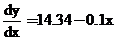Solution y = 1400 + 14.34x -0.05 x2 = negative value ie. Therefore the given function has a maximum point. Physical Optimum i.e 14.34-0.1x = 0 -0.1 x = -14.34 x = kgs/hectare therefore the physical optimum level of nitrogen is 143.4 kgs/hectare. Therefore the maximum yield is Y = 1400 + 14.34(143.4) -0.05(143.4)2 = 2428.178 kgs/ hectare. Economic optimum Given Price of nitrogen per kg = Px = 5 Price of yield per kg = Py = 2 Therefore 14.34-0.1x = 28.68 - 0.2 x = 5 - 0.2 x = 5 - 28.68 x = kgs/hectare therefore the economic optimum level of nitrogen is 118.4 kgs/hectare. Therefore the maximum yield is Y = 1400 + 14.34(118.4) -0.05(118.4)2 = 2396.928 kgs/ hectare. Maxima and Minima of several variables with constraints and without constraints Consider the function of several variables y = f (x1, x2……….xn) where x­1, x2 …………..xn are n independent variables and y is the dependent variable.

Working Rule

Step 1: Find all the first order partial derivatives of y with respect to x1, x2, x3 ……xn..__ (ie)

. . . .

Step 2

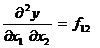
Find all the second order partial derivatives of y with respect to x1, x2, x3 ….xn and they are given as follows. and so on

Step: 3

Construct an Hessian matrix which is formed by taking all the second order partial derivatives is given by

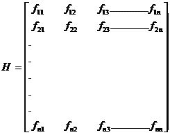
H is a symmetric matrix.

Step: 4

Consider the following minors of order 1, 2, 3 ……….

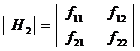
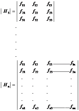
Steps: 5

The necessary condition for finding the maximum or minimum

Equate the first order derivative to zero (i.e) f1 = f2 = ……..fn = 0 and find the value of x1, x2, ……..xn.

Steps: 6

Substitute the values x1, x2 ……..xn in the Hessian matrix. Find the values of If 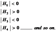Then the function is maximum at x1, x2 ……..xn. If then the function is minimum at x1, x2……. xn.

Steps: 7

Conditions

| Maximum | Minimum ---|---|--- First | f1 = f2 = f3 = fn = 0 | f1 = 0, f2 = 0 ……. fn = 0 Second | ………. |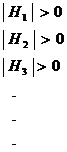

Note : If the second order conditions are not satisfied then they are called saddle point.

Problem

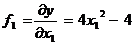
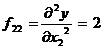
Find the maxima (or) minima if any of the following function. Solution Step 1: The first order partial derivatives are Step 2: The second order partial derivatives are 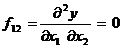Step 3: The Hessian matrix is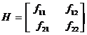

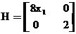4. Equate f1, f2 = 0 f1 Þ 4x12 - 4 = 0 x12 = 1 x1 = 1 x1 = 1, x1 = -1 f2 Þ 2 x 2 + 8=0 2 x2 = - 8 x2 = - 4 The stationary points are (1,- 4) & (-1, - 4) At the point (1, - 4) the Hessian matrix will be H =

| H1| = | 8| > 0 | H2| = = 16 > 0 Since the determinant H1 and H2 are positive the function is minimum at (1,- 4). The minimum value at x1 = 1 & x2 = - 4 is obtained by substituting the values in (1) y = (1) 3 + (- 4)2 – 4 (1) + 8 (- 4) y = + 16 – 4 - 32 y = - 20 y = = The minimum value is At the point (-1, - 4) H = | H1 | = | - 8 | = - 8 < 0 | H 2| = - 16 < 0 Both the conditions are not satisfied. Hence the point (-1, - 4) gives a saddle point.

Economic Optimum

For finding the Economic Optimum we equate the first order derivative f1 . f 2 . . . . fn to the inverse ratio of the unit prices. (ie) f1 = f2 = ………….. fn =

where Px1 , Px2,… Pxn and Py are the unit prices of x1, x2 ….. xn and y. These are the first order condition. The economic optimum & the physical optimum differ only in the first order conditions. The other procedures are the same.

Maxima & Minima of several variables under certain condition with constraints.

Consider the response function y = f (x1, x2 ….xn ) subject to the constraint f (x1, x2…..xn ) =0 The objective function is Z= f(x1, x2, …xn) + l[f(x1, x2, …xn)] where l is called the Lagrange’s multiplies. The partial derivatives are for i = 1, 2 ….. n. i, j = 1., 2 …. n. i = 1, 2 ….. n. Now form the Bordered Hessian Matrix as follows. Bordered Hessian 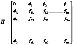[Since this extra row & column is on the border of the matrix 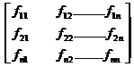.So we call it as Bordered Hessian matrix and it is denoted by ] Here minor as are

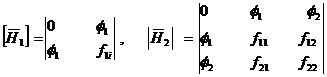
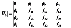and so on.

Conditions	Maxima	Minima
First Order	f1=f2= f3 = ….fn =0	f1= f2 = f3 …… fn = 0
Second Order

Problem

Consider a consumer with a simple utility function U = f(x, y) = 4xy – y2 . If this __ consumer can at most spend only Rs. 6/- on two goods x and y and if the current prices are Rs. 2/- per unit of x and Rs.1/- per unit of y. Maximize the function.

---|---

Summary Cheat Sheet

• Focus on core formulas, definitions, and solved patterns from this lesson.
• Practice stepwise derivations and numerical substitutions carefully.
• Connect each concept to practical agricultural problem-solving contexts.

References

1 source

Primary classroom notes and standard BSc Agriculture applied mathematics references.