💻 Models
Models.
This lesson covers core applied mathematics concepts and their agricultural applications for BSc Agriculture learners.
MATHS :: Lecture 14 :: Model
Definition
Model
A mathematical model is a representation of a phenomena by means of mathematical equations. If the phenomena is growth, the corresponding model is called a growth model. Here we are going to study the following 3 models. 1. linear model 2. Exponential model 3. Power model
1. Linear model
The general form of a linear model is y = a+bx. Here both the variables x and y are of degree 1. To fit a linear model of the form y=a+bx to the given data. Here a and b are the parameters (or) constants of the model. Let (x1 , y1) (x2 , y2)…………. (xn , yn) be n pairs of observations. By plotting these points on an ordinary graph sheet, we get a collection of dots which is called a scatter diagram.
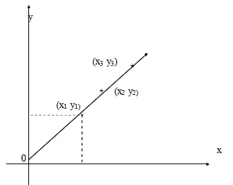
There are two types of linear models (i) y = a+bx (with constant term) (ii) y = bx (without constant term) The graphs of the above models are given below :
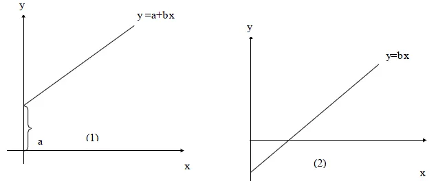
‘a’ stands for the constant term which is the intercept made by the line on the y axis. When x =0, y =a ie ‘a’ is the intercept, ‘b’ stands for the slope of the line . Eg:1. The table below gives the DMP(kgs) of a particular crop taken at different stages; fit a linear growth model of the form w=a+bt, and find the value of a and b from the graph.
| t (in days) ; | 0 | 5 | 10 | 20 | 25 |
|---|---|---|---|---|---|
| DMP w: (kg/ha) | 2 | 5 | 8 | 14 | 17 |
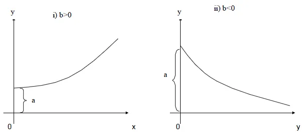
2. Exponential model
This model is of the form y = aebx where a and b are constants to be determined
The graph of an exponential model is given below.
‘a’ stands for the constant term which is the intercept made by the line on the y axis. When x =0, y =a ie ‘a’ is the intercept, ‘b’ stands for the slope of the line . Eg:1. The table below gives the DMP(kgs) of a particular crop taken at different stages; fit a linear growth model of the form w=a+bt, and find the value of a and b from the graph.
| t (in days) ; | 0 | 5 | 10 | 20 | 25 |
|---|---|---|---|---|---|
| DMP w: (kg/ha) | 2 | 5 | 8 | 14 | 17 |
2. Exponential model
This model is of the form y = aebx where a and b are constants to be determined
The graph of an exponential model is given below.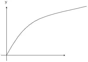 o x
Example: Fit the power function for the following data
o x
Example: Fit the power function for the following data
| x | 0 | 1 | 2 | 3 |
|---|---|---|---|---|
| y | 0 | 2 | 16 | 54 |
Crop Response models The most commonly used crop response models are
- Quadratic model
- Square root model
Quadratic model The general form of quadratic model is y = a + b x + c x2
 The parabolic curve bends very sharply at the maximum or minimum points.
Example
Draw a curve of the form y = a + b x + c x2 using the following values of x and y
| x | 0 | 1 | 2 | 4 | 5 | 6 |
|---|---|---|---|---|---|---|
| y | 3 | 4 | 3 | -5 | -12 | -21 |
Square root model
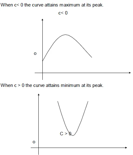
The standard form of the square root model is y = a +b + cx
When c is negative the curve attains maximum
+ cx
When c is negative the curve attains maximum
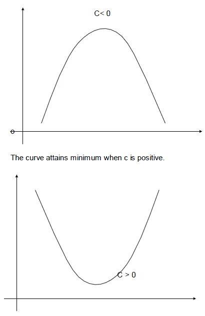
At the extreme points the curve bends at slower rate
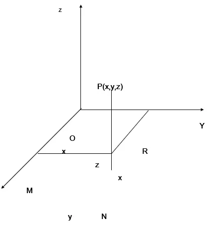
Three dimensional Analytical geometry
Let OX ,OY & OZ be mutually perpendicular straight lines meeting at a point O. The extension of these lines OX1, OY1 and OZ1 divide the space at O into octants(eight). Here mutually perpendicular lines are called X, Y and Z co-ordinates axes and O is the origin. The point P (x, y, z) lies in space where x, y and z are called x, y and z coordinates respectively.
Distance between two points
The distance between two points A(x1,y1,z1) and B(x2,y2,z2) is
dist AB =  In particular the distance between the origin O (0,0,0) and a point P(x,y,z) is
OP =
In particular the distance between the origin O (0,0,0) and a point P(x,y,z) is
OP = 
The internal and External section __
Suppose P(x1,y1,z1) and Q(x2,y2,z2) are two points in three dimensions.

P(x1,y1,z1) A(x, y, z) Q(x2,y2,z2) The point A(x, y, z) that divides distance PQ internally in the ratio m1:m2 is given by
A = 
Similarly
P(x1,y1,z1) and Q(x2,y2,z2) are two points in three dimensions.

P(x1,y1,z1) Q(x2,y2,z2) A(x, y, z)
The point A(x, y, z) that divides distance PQ externally in the ratio m1:m2 is given by
A = 
If A(x, y, z) is the midpoint then the ratio is 1:1
A = 
Problem
Find the distance between the points P(1,2-1) & Q(3,2,1)
PQ=  =
= =
= =2
=2
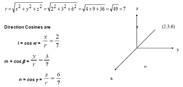
Direction Cosines
Let P(x, y, z) be any point and OP = r. Let a,b,g be the angle made by line OP with OX, OY & OZ. Then a,b,g are called the direction angles of the line OP. cos a, cos b, cos g are called the direction cosines (or dc’s) of the line OP and are denoted by the symbols I, m ,n.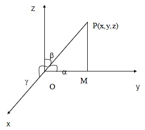
Result
By projecting OP on OY, PM is perpendicular to y axis and the also OM = y
 Similarly,
 (i.e) l =
 m =
m =  n =
n =  _l2 + m2 + n2_ =
  (
( Distance from the origin)
\ l2 + m2 + n2 =
Distance from the origin)
\ l2 + m2 + n2 =  l2 + m2 + n2 = 1
(or) cos2a + cos2b + cos2g = 1.
l2 + m2 + n2 = 1
(or) cos2a + cos2b + cos2g = 1.
Note
The direction cosines of the x axis are (1,0,0) The direction cosines of the y axis are (0,1,0) The direction cosines of the z axis are (0,0,1)
Direction ratios
Any quantities, which are proportional to the direction cosines of a line, are called direction ratios of that line. Direction ratios are denoted by a, b, c.
If l, m, n are direction cosines an a, b, c are direction ratios then
a µ l, b µ m, c µ n
(ie ) a = kl, b = km, c = kn
(ie)  (Constant)
(or)
(Constant)
(or)  (Constant)
To find direction cosines if direction ratios are given
If a, b, c are the direction ratios then direction cosines are

 l =
l =
 similarly m =
 (1)
n =
(1)
n =
l2+m2+n2 = (ie) 1 =
 Taking square root on both sides
K =
Taking square root on both sides
K =  !lec14_clip_image044.gif
Problem
1. Find the direction cosines of the line joining the point (2,3,6) & the origin.
Solution
By the distance formula
2. Direction ratios of a line are 3,4,12. Find direction cosines
Solution
Direction ratios are 3,4,12
(ie) a = 3, b = 4, c = 12
Direction cosines are
l =  m =
m =  n =
n = 
Note
- The direction ratios of the line joining the two points A(x1, y1, z1) & B (x2, y2, z2) are (x2 – x1, y2 – y1, z2 – z1)
- The direction cosines of the line joining two points A (x1, y1, z1) &
B (x2, y2, z2) are 
---|---
Summary Cheat Sheet
- Focus on core formulas, definitions, and solved patterns from this lesson.
- Practice stepwise derivations and numerical substitutions carefully.
- Connect each concept to practical agricultural problem-solving contexts.
References
1 source
References
Primary classroom notes and standard BSc Agriculture applied mathematics references.
Lesson Doubts
Ask questions, get expert answers