🎛 Production Function — Types, Algebraic Models and Agricultural Applications
Master the production function concept — how farm inputs transform into crop output. Covers continuous vs discrete, short run vs long run, and algebraic models (Linear, Quadratic, Cubic, Cobb-Douglas) with agricultural examples, comparison tables, and exam mnemonics.
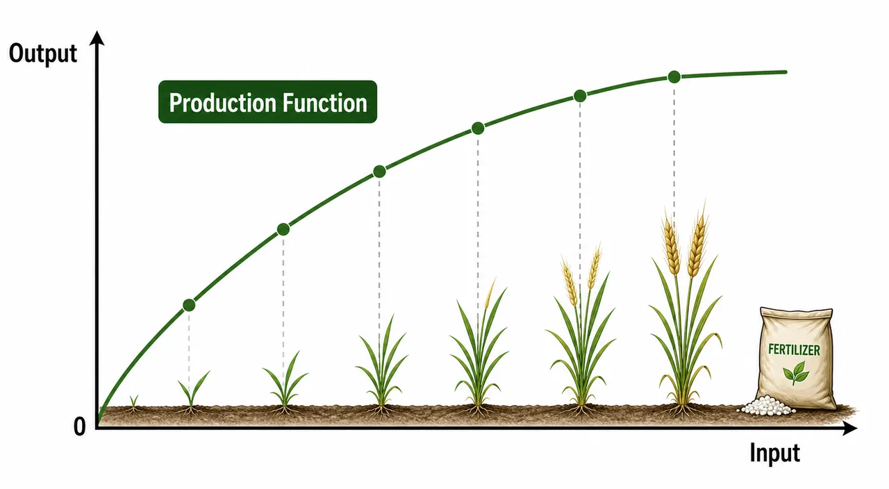
A wheat farmer applies 50 kg of urea per hectare and harvests 30 quintals. When the dose rises to 100 kg, yield jumps to 45 quintals. At 150 kg, it barely reaches 50 quintals. Notice the pattern: each additional 50 kg of urea adds less and less grain. This systematic relationship between the quantity of input used and the resulting output is called a production function.
The real farm question is not just whether output rises, but how fast it rises, when the response begins to slow, and when extra input stops making economic sense. That is why production functions are so important: they turn field observation into a decision rule.
What Is a Production Function?
A production function is a technical and mathematical relationship showing how the quantity of output depends on the quantities of inputs used, given a fixed level of technology and a specific time period.
Pro Content Locked
Upgrade to Pro to access this lesson and all other premium content.
₹99 charged monthly · Cancel anytime
- All Agriculture & Banking Courses
- AI Lesson Questions (100/day)
- AI Doubt Solver (50/day)
- Glows & Grows Feedback (30/day)
- AI Section Quiz (20/day)
- 22-Language Translation (100/day)
- Recall Questions (20/day)
- AI Quiz (15/day)
- AI Quiz Paper Analysis (100/day)
- AI Step-by-Step Explanations (100/day)
- Spaced Repetition Recall (FSRS)
- AI Tutor
- Immersive Text Questions
- Audio Lessons — Hindi & English
- Mock Tests & Previous Year Papers
- Summary & Mind Maps
- XP, Levels, Leaderboard & Badges
- Generate New Classrooms
- Voice AI Teacher (AgriDots Live)
- AI Revision Assistant
- Knowledge Gap Analysis
- Interactive Revision (LangGraph)
🔒 Secure via Razorpay · Cancel anytime · No hidden fees
A wheat farmer applies 50 kg of urea per hectare and harvests 30 quintals. When the dose rises to 100 kg, yield jumps to 45 quintals. At 150 kg, it barely reaches 50 quintals. Notice the pattern: each additional 50 kg of urea adds less and less grain. This systematic relationship between the quantity of input used and the resulting output is called a production function.
The real farm question is not just whether output rises, but how fast it rises, when the response begins to slow, and when extra input stops making economic sense. That is why production functions are so important: they turn field observation into a decision rule.
What Is a Production Function?
A production function is a technical and mathematical relationship showing how the quantity of output depends on the quantities of inputs used, given a fixed level of technology and a specific time period.
In simple terms: Input goes in, output comes out — the production function tells you exactly how much.
Agricultural example: The relationship between kg of nitrogen applied per hectare and quintals of paddy harvested is a production function.
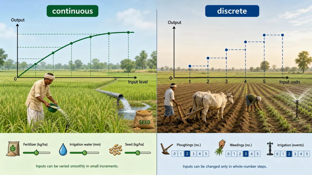
Types Based on Input Divisibility
The first classification depends on whether the input can be measured in fractions or only in whole numbers.
Continuous Production Function
Obtained when inputs can be divided into smaller measurable units. The resulting curve is smooth and unbroken.
Agricultural examples: Fertilizer (apply 10 kg, 20 kg, 25.5 kg), seed (any weight), irrigation water (any volume), animal feed (any quantity).
Discrete (Discontinuous) Production Function
Obtained when inputs are used in whole numbers only and cannot be split into fractions. The function appears as distinct points rather than a smooth curve.
Agricultural examples: Number of ploughings (1, 2, 3 — not 1.5), number of weedings, number of irrigation events.
| Feature | Continuous | Discrete |
|---|---|---|
| Input type | Measurable, divisible | Counted, indivisible |
| Graph shape | Smooth curve | Distinct points |
| Agricultural examples | Fertilizer, seed, water, feed | Ploughings, weedings, irrigation events |
Exam Tip — Mnemonic: "Measured = Continuous. Counted = Discrete." (Think: a measuring cup pours smoothly; counting fingers gives jumps.)
Short Run vs Long Run Production Function
The second classification depends on whether any input remains fixed.
Short Run Production Function (SRPF)
At least one input is fixed. The farmer adjusts only variable inputs within a single season.
Y = f(X1 | X2, X3, ..., Xn)
The vertical bar separates the variable input (X1) from the fixed inputs. This function demonstrates the Law of Diminishing Returns (Law of Variable Proportions).
Agricultural example: A farmer owns 2 hectares of land (fixed). By varying the amount of nitrogen fertilizer (variable), the farmer observes how wheat yield changes. Land cannot be increased within the crop season.
Long Run Production Function (LRPF)
All inputs can be varied — nothing is fixed.
Y = f(X1, X2, X3, ..., Xn)
This function demonstrates Returns to Scale.
Agricultural example: Over several years, a farmer buys more land, purchases new machinery, hires permanent labour, and increases all inputs proportionally.
| Feature | Short Run (SRPF) | Long Run (LRPF) |
|---|---|---|
| Fixed inputs | At least one | None |
| Variable inputs | Some | All |
| Related law | Law of Diminishing Returns | Returns to Scale |
| Notation | Y = f(X1 | X2, X3, ..., Xn) | Y = f(X1, X2, X3, ..., Xn) |
| Agricultural example | Varying fertilizer on fixed land in one season | Expanding entire farm over several years |
| Time horizon | Within one crop season | Across multiple seasons or years |
Exam Tip — Mnemonic: "Short run = Something fixed. Long run = Liberated (all inputs free to change)."
Three Ways to Express a Production Function
A production function can be presented in three forms — tabular, graphical, and algebraic. Each serves a different purpose.
1. Tabular Form
A simple table listing input levels and the corresponding output. Easy to read but limited to the specific data points collected.
Agricultural example — Nitrogen and Wheat Yield:
| Nitrogen (kg/ha) | Wheat Yield (q/ha) | Additional Yield from Last 20 kg |
|---|---|---|
| 0 | 15 | — |
| 20 | 25 | +10 |
| 40 | 33 | +8 |
| 60 | 39 | +6 |
| 80 | 43 | +4 |
| 100 | 45 | +2 |
Notice how each additional 20 kg of nitrogen adds progressively less yield — a classic example of diminishing returns in agriculture.
| Input (X) | Output (Y) |
|---|---|
| 0 | 2 |
| 10 | 5 |
| 20 | 11 |
| 30 | 18 |
| 40 | 25 |
2. Graphical Form
Input is plotted on the horizontal axis (X) and output on the vertical axis (Y). The shape of the curve reveals whether returns are increasing, constant, or diminishing.
Agricultural use: Soil scientists and agronomists plot fertilizer response curves this way to recommend optimal doses for different crops.
3. Algebraic Form
The most precise way — an equation that allows prediction for any input level, not just observed data points.
General form:
Y = f(X)
Where:
- Y = dependent variable (output — crop yield, milk production)
- X = independent variable (input — seed, fertilizer, feed)
- f = "function of"
Multiple inputs:
Y = f(X1, X2, X3, X4, ..., Xn)
Single variable function (one input varies, rest fixed):
Y = f(X1 | X2, X3, ..., Xn)
Multiple variable inputs with some fixed:
Y = f(X1, X2 | X3, X4, ..., Xn)
Algebraic Models of Production Functions
Moving from simple to complex, here are the five key algebraic models used in agriculture.
1. Linear Production Function
Y = a + bX
| Symbol | Meaning | Agricultural Interpretation |
|---|---|---|
| Y | Output | Yield of wheat (q/ha) |
| a | Constant (intercept) | Yield from fixed factors alone (no variable input applied) |
| b | Coefficient (slope) | Additional yield per unit of input — always the same |
| X | Input | Kg of fertilizer applied |
Each additional unit of input always adds the same amount to output — constant marginal returns. This is rarely realistic across a wide input range in agriculture.
Agricultural example: If Y = 10 + 0.5X, then without fertilizer the yield is 10 q/ha, and every additional kg of fertilizer adds exactly 0.5 quintal — whether it is the 1st kg or the 100th kg.
2. Quadratic Production Function
Y = a + bX + cX^2
The squared term (cX^2) allows for diminishing returns. When c is negative, the curve bends downward, capturing the realistic pattern where additional input eventually adds less and less output.
Agricultural example: Y = 10 + 2X - 0.01X^2 for nitrogen and wheat yield. Initially yield rises fast, but each additional kg of nitrogen contributes less. This is the most commonly used model for fertilizer response studies in India.
3. Square Root Production Function
Y = a + b sqrt(X1) + cX2
The square root term increases at a decreasing rate, naturally modelling diminishing returns without needing a negative coefficient.
Agricultural example: Modelling paddy yield response to irrigation water — initial water additions dramatically boost yield, but beyond a point, additional water adds little.
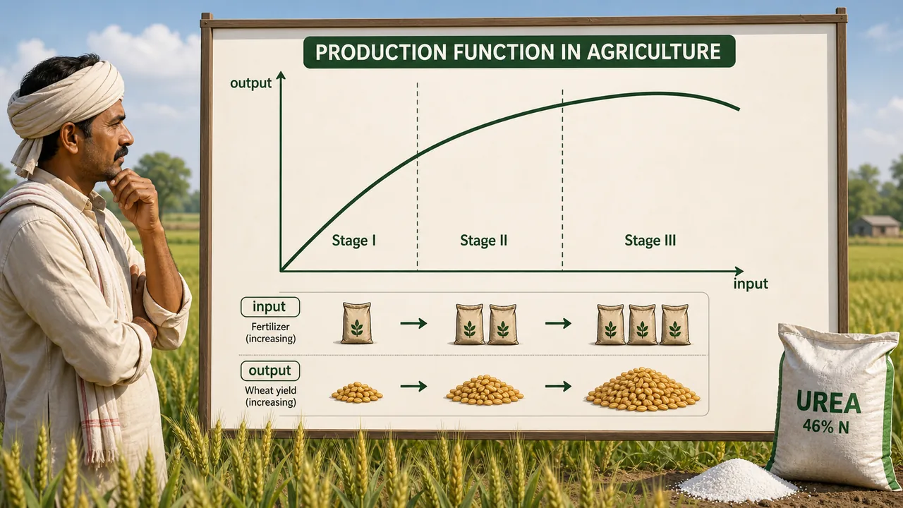
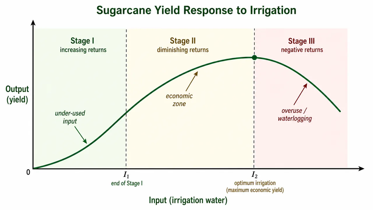
4. Cubic Production Function
Y = a0 + a1X + a2X^2 + a3X^3
The most flexible single-variable form — capable of showing all three stages of production (increasing returns, diminishing returns, and negative returns) within a single equation.
Agricultural example: Modelling sugarcane yield response to irrigation from water-starved conditions (Stage I: increasing returns) through optimal watering (Stage II: diminishing returns) to waterlogged conditions (Stage III: negative returns).
5. Cobb-Douglas Production Function
Propounded by Cobb and Douglas, this function expresses output as a product of labour and capital raised to powers. (UPPSC 2021)
Q = K L^alpha C^beta
Where: Q = Output, K = Constant, L = Labour, C = Capital, alpha and beta = output elasticities (the percentage change in output for a 1% change in each input).
In the original solution by Cobb-Douglas, the share of labour was 3/4 and that of capital was 1/4:
Y = K L^(3/4) C^(1/4)
Returns to Scale from Cobb-Douglas
The sum of the exponents (alpha + beta) determines the type of returns to scale:
| Condition | Type of Returns | Meaning | Agricultural Example |
|---|---|---|---|
| alpha + beta = 1 | Constant Returns to Scale (CRS) | Doubling all inputs exactly doubles output | A 2-hectare farm expanded to 4 hectares with proportional inputs gets exactly double yield |
| alpha + beta > 1 | Increasing Returns to Scale (IRS) | Doubling all inputs more than doubles output | Large mechanised farm benefits from economies of scale |
| alpha + beta < 1 | Decreasing Returns to Scale (DRS) | Doubling all inputs less than doubles output | Very large farm faces management strain, supervision difficulties |
Key properties:
- When alpha + beta = 1, it is a Linear Homogeneous Production Function (linear in logarithmic form, not natural scale).
- Cobb-Douglas has constant elasticity of substitution, making it widely used for its mathematical convenience.
Exam Tip — Mnemonic: "Sum = 1, CRS done!" If alpha + beta = 1, it is CRS. Greater than 1 = IRS (Increasing). Less than 1 = DRS (Decreasing). Remember the alphabetical order: C-D-I maps to =1, <1, >1.
Comparison of All Algebraic Models
| Type | Equation | Returns Pattern | Stages Shown | Best Agricultural Use |
|---|---|---|---|---|
| Linear | Y = a + bX | Constant returns only | None clearly | Rough approximation over narrow input range |
| Quadratic | Y = a + bX + cX^2 | Diminishing returns | II only | Fertilizer-yield response curves (most common in India) |
| Square Root | Y = a + b sqrt(X) + cX2 | Diminishing returns | II only | Crop response to irrigation water |
| Cubic | Y = a0 + a1X + a2X^2 + a3X^3 | All three stages | I, II, III | Complete input-response modelling (sugarcane, paddy) |
| Cobb-Douglas | Q = K L^alpha C^beta | Depends on alpha + beta | Depends on exponents | Farm-level productivity analysis, policy research |
Summary Cheat Sheet
| Concept / Topic | Key Details / Explanation |
|---|---|
| Production Function | Mathematical relationship between input quantities and output quantity, given fixed technology and time |
| Continuous PF | Inputs are measurable and divisible (fertilizer, seed, water); smooth curve |
| Discrete PF | Inputs are counted in whole numbers (ploughings, weedings, irrigations); distinct points |
| Short Run PF (SRPF) | At least one input fixed; Y = f(X1 / X2...Xn); demonstrates Law of Diminishing Returns |
| Long Run PF (LRPF) | All inputs variable; Y = f(X1, X2...Xn); demonstrates Returns to Scale |
| Tabular Form | Input-output data in a table; easy to read but limited to observed data points |
| Graphical Form | Input on X-axis, output on Y-axis; curve shape reveals return pattern |
| Algebraic Form | Y = f(X); most precise representation; allows prediction for any input level |
| Linear PF | Y = a + bX; constant marginal returns; each unit adds same output; unrealistic over wide range |
| Quadratic PF | Y = a + bX + cX^2; captures diminishing returns (c is negative); most commonly used in fertilizer studies |
| Square Root PF | Y = a + b sqrt(X) + cX2; naturally models diminishing returns via square root term |
| Cubic PF | Y = a0 + a1X + a2X^2 + a3X^3; shows all three stages of production; most flexible single-variable form |
| Cobb-Douglas PF | Q = K L^alpha C^beta; propounded by Cobb and Douglas; alpha + beta determines returns to scale |
| Original Cobb-Douglas | Labour share = 3/4, Capital share = 1/4 (Y = K L^(3/4) C^(1/4)) |
| alpha + beta = 1 | Constant Returns to Scale (CRS); doubling inputs exactly doubles output |
| alpha + beta > 1 | Increasing Returns to Scale (IRS); doubling inputs more than doubles output |
| alpha + beta < 1 | Decreasing Returns to Scale (DRS); doubling inputs less than doubles output |
| Linear Homogeneous PF | When alpha + beta = 1; linear in logarithmic form (not natural scale) |
| Mnemonic: Sum = 1, CRS done! | alpha + beta: = 1 (CRS), > 1 (IRS), < 1 (DRS) |
| UPPSC 2021 | Cobb-Douglas production function was asked in UPPSC 2021 |