🏦Production Economics — Principles, Problems and Laws of Returns

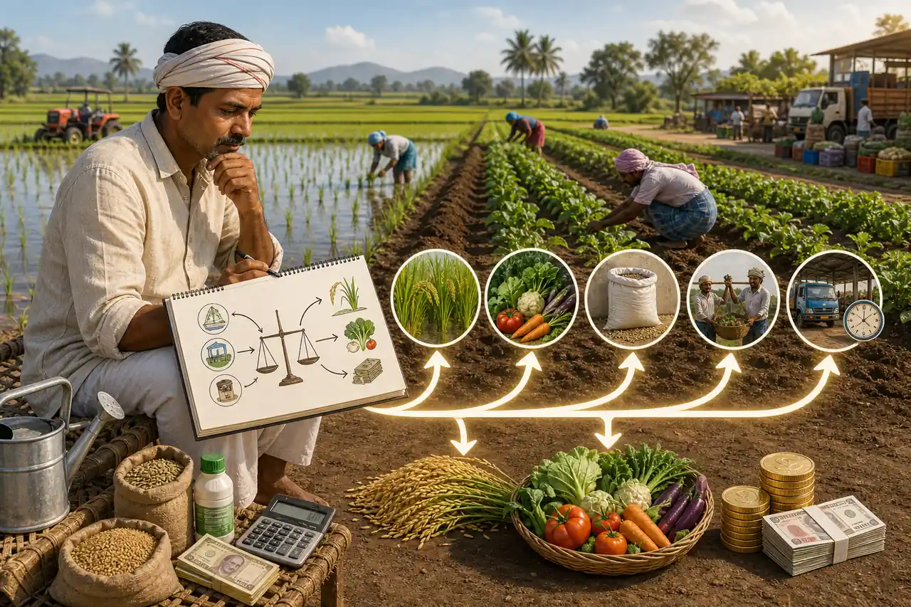
A marginal farmer in Bihar has 1 hectare of land, limited capital, and family labour. Should she grow paddy alone or split the land between paddy and vegetables? How much fertilizer should she use? These are the exact questions agricultural production economics helps answer.

---

What Is Agricultural Production Economics?

Agricultural production economics is a specialized branch of agricultural economics concerned with the choice of production patterns and resource use to maximize the objectives of farmers, their families, and the nation — all within a framework of limited resources.

It answers two fundamental questions:

1. How to organize resources to maximize production of a single commodity? (Choosing among alternative ways of using resources.)
2. What combination of commodities to produce for best results?

Definition: Agricultural production economics is an applied field of science wherein the principles of choice are applied to the use of capital, labour, land, and management resources in the farming industry.

---

Goals of Production Economics

Goal	Focus	Agricultural Example
Guide individual farmers	Help each farmer use resources most efficiently	Advising a wheat farmer on optimal fertilizer dose
Efficient national resource use	Deploy the country’s agricultural resources for maximum social benefit	Government deciding how to allocate irrigation water across districts

---

Subject Matter

Production economics deals with productivity — the use and income from productive inputs (land, labour, capital, management). Specifically, it covers:

Area	Question It Answers	Agricultural Example
Resource use efficiency	Are resources being used to their full potential?	Is the farmer applying fertilizer at the right rate?
Resource combination	What is the best mix of inputs?	Optimal ratio of labour to machinery for harvesting
Resource allocation	How should limited resources be distributed?	Dividing irrigation water between wheat and mustard fields
Resource management	How should resources be maintained over time?	Soil conservation practices to sustain land productivity
Resource administration	How should resource use be organized?	Cooperative management of a shared cold storage

Broader topics include: methods of production, enterprise combination, farm size, returns to scale, leasing, production possibilities, farming efficiency, soil conservation, credit and capital use, and risk and uncertainty in decision-making.

Key principle: Any agricultural problem involving resource allocation and marginal productivity analysis falls within the scope of production economics.

---

Four Objectives of Production Economics

1. Determine and define the conditions for optimum use of resources.
2. Measure the gap between existing resource use and the optimum.
3. Analyze the factors responsible for the current production pattern.
4. Prescribe methods to move from existing use to the optimum level.

Mnemonic — D-M-A-P: “Define the optimum, Measure the gap, Analyze the cause, Prescribe the cure.”

---

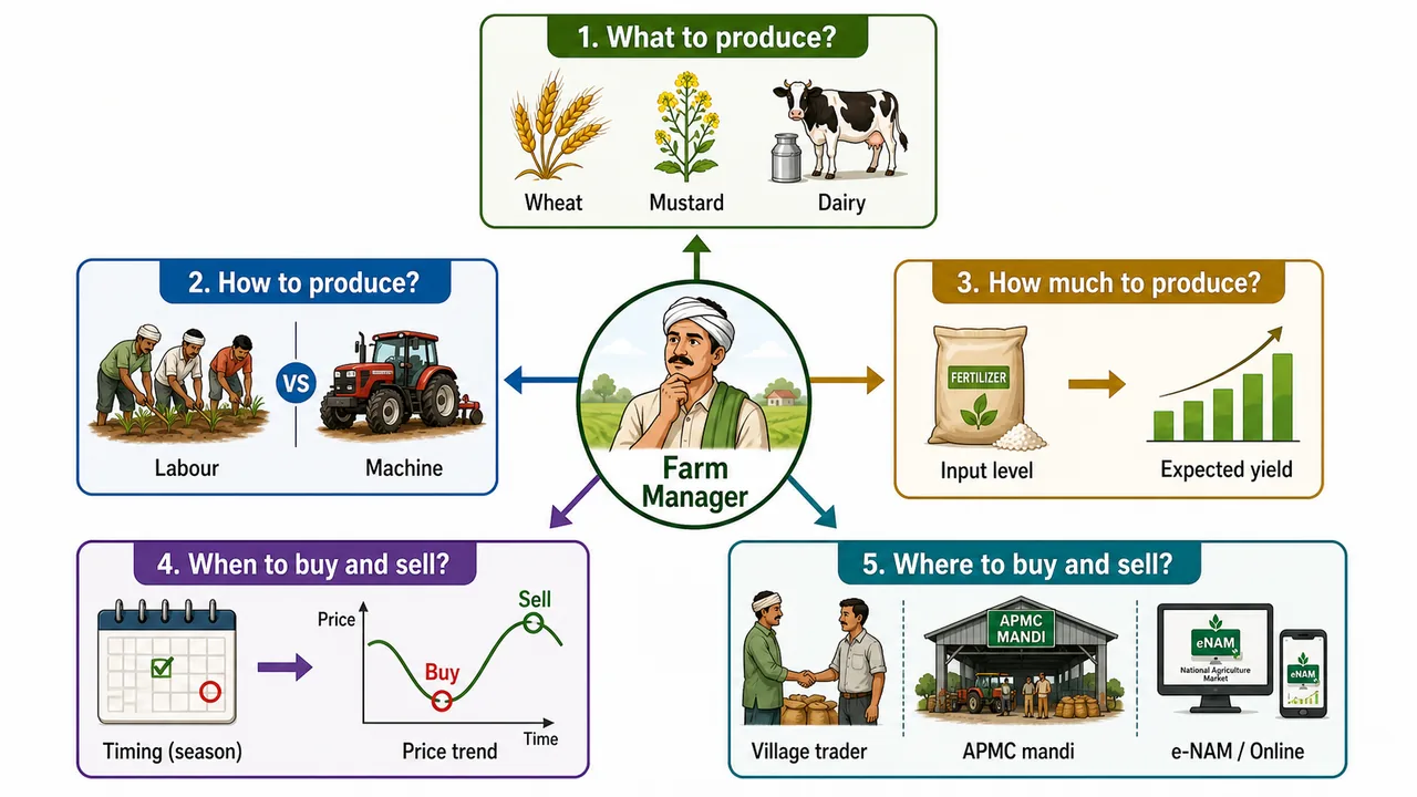
Five Basic Production Problems

Every farmer or farm manager faces these five decision problems:

1. What to Produce? (Product-Product Relationship)

Selecting the combination of crops and livestock enterprises. Should the farm produce only crops, only livestock, or both? Which crops and rotations?

Example: A farmer in UP must decide between growing wheat alone or a wheat-mustard combination to maximize profit.

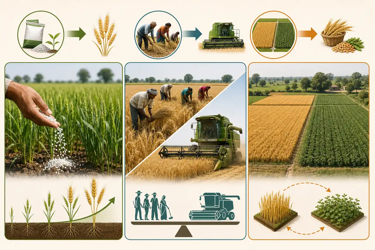
2. How to Produce? (Factor-Factor Relationship)

Choosing the right combination of inputs to minimize cost for a given level of output. Should the farm use capital-intensive or labour-intensive technology?

Example: Harvesting paddy — use a combine harvester (capital-intensive) or hire manual labourers (labour-intensive)? The choice depends on relative costs.

3. How Much to Produce? (Factor-Product Relationship)

Deciding the level of each input to determine output and profit. How much fertilizer, irrigation, seed, and labour to use?

Example: Should a cotton farmer apply 80 kg or 120 kg of nitrogen per hectare? The answer depends on how much extra yield each additional kg produces versus its cost.

4. When to Buy and Sell?

Agricultural markets are seasonal — input and output prices fluctuate throughout the year. Timing decisions directly affect profitability.

Example: Selling wheat immediately after harvest (April) when prices are low vs storing and selling in August when prices rise.

5. Where to Buy and Sell?

Choosing the market that offers the best prices for outputs and lowest costs for inputs.

Example: Selling onions at the village trader’s shop vs the APMC mandi vs an e-NAM portal — each offers different prices.

Problem	Relationship Type	Core Decision	Agricultural Example
What to produce?	Product-Product	Enterprise selection	Wheat vs mustard vs dairy
How to produce?	Factor-Factor	Input combination	Combine harvester vs manual labour
How much to produce?	Factor-Product	Input level	80 kg vs 120 kg nitrogen/ha
When to buy/sell?	Timing	Market timing	Sell wheat in April vs August
Where to buy/sell?	Market choice	Market selection	Village shop vs APMC mandi vs e-NAM

Exam Tip: The first three problems correspond to the three basic production relationships (product-product, factor-factor, factor-product). Questions 4 and 5 deal with market timing and location.

---

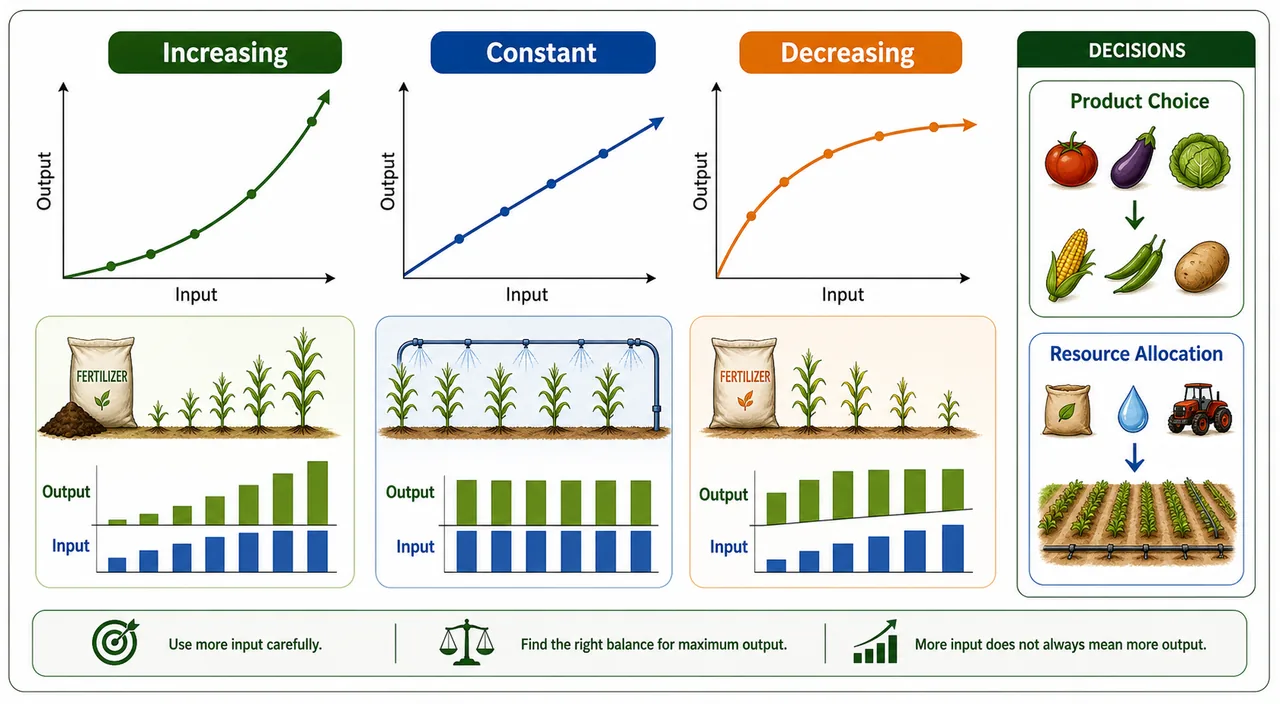
Laws of Returns

Production results from the cooperative working of land, labour, capital, and management. The laws of returns describe what happens to output when one input is varied while others remain fixed.

---

Law of Increasing Returns (Increasing Marginal Productivity)

Each successive unit of variable input adds more and more to total output than the previous unit.

Why it happens: The fixed resources are under-utilized initially. Adding variable input allows better use of fixed resources.

Cost implication: Cost per unit of additional output falls — hence also called the Law of Decreasing Costs.

Agricultural example: On a well-prepared 1-hectare field, the first 20 kg of nitrogen adds 8 quintals of wheat, the second 20 kg adds 10 quintals, and the third 20 kg adds 12 quintals. Each dose is more productive because the soil’s potential is progressively unlocked.

• The production curve is convex to the origin (curves upward).

Algebraic condition:

Each additional unit of input produces more output than the previous unit. MPP(n) > MPP(n-1)

---

Law of Constant Returns (Constant Marginal Productivity)

Each additional unit of variable input produces an equal amount of additional output. Total output rises in a straight line.

Cost implication: Cost per additional unit of output remains the same — hence also called the Law of Constant Costs.

Note: Constant returns is uncommon in agriculture because land is a constraining fixed factor.

Agricultural example: Each additional hired labourer picks exactly 50 kg of tea leaves per day (within a narrow range of 3-5 workers on a small plot).

• The production curve is a straight line (linear).

Algebraic condition:

MPP(n) = MPP(n-1)

---

Law of Decreasing Returns (Diminishing Marginal Productivity)

Each additional unit of variable input adds less and less to total output than the previous unit.

Why it happens: As more variable input is added to a fixed resource, each additional unit has less of the fixed resource to work with.

Cost implication: Cost per additional unit of output rises — hence also called the Law of Increasing Costs.

This is the most common law in agriculture because land is the primary fixed factor.

Input (X)	Output (Y)	ΔX	ΔY	ΔY/ΔX = MPP
1	25	1	25	25/1 = 25
2	45	1	20	20/1 = 20
3	60	1	15	15/1 = 15
4	70	1	10	10/1 = 10
5	75	1	5	5/1 = 5

Agricultural example: On 1 hectare of paddy — the first 20 kg of nitrogen adds 12 quintals, the second 20 kg adds 8 quintals, the third 20 kg adds only 4 quintals. The soil’s capacity to respond is getting saturated.

• The production curve is concave to the origin (curves downward).

Algebraic condition:

MPP(n) < MPP(n-1)

---

Comparison of the Three Laws of Returns

Feature	Increasing Returns	Constant Returns	Decreasing Returns
MPP trend	Rising	Unchanged	Falling
TPP curve shape	Convex to origin	Straight line	Concave to origin
Cost per unit of output	Decreasing	Constant	Increasing
Also called	Law of Decreasing Costs	Law of Constant Costs	Law of Increasing Costs
Common in agriculture?	Initial stage only	Rare	Very common
Agricultural example	First doses of fertilizer on nutrient-deficient soil	Narrow range of labour on small tea plot	Heavy fertilizer doses on already-fertilized field

Exam Tip — Mnemonic “ICDs”: Increasing returns = Decreasing costs. Constant returns = Constant costs. Decreasing returns = Increasing costs. The returns and costs move in opposite directions.

---

Three Basic Production Relationships

All farm production problems can be analyzed through three fundamental relationships:

Relationship	Variables	Core Question	Agricultural Example
Factor-Product	One input vs one output	How much input to use? How much to produce?	How much urea for wheat?
Factor-Factor	Two inputs vs one output	What input combination minimizes cost?	Labour vs machinery for harvesting
Product-Product	One input vs two outputs	What output combination maximizes profit?	Wheat vs gram on the same land

Exam Tip: “Factor = input, Product = output.” Factor-Product means input-output. Factor-Factor means input-input. Product-Product means output-output.

---

Summary Table

Concept	Key Point
Production Economics	Applied science of choice — optimizing farm resource use
Two fundamental questions	How to maximize single-commodity output? What commodity mix to produce?
Goals	Guide individual farmers + efficient national resource use
Subject matter areas	Resource efficiency, combination, allocation, management, administration
Four objectives	Define optimum, measure gap, analyze causes, prescribe methods (D-M-A-P)
Five production problems	What, How, How much, When, Where
Product-Product relationship	What to produce (enterprise selection)
Factor-Factor relationship	How to produce (input combination)
Factor-Product relationship	How much to produce (input level)
Increasing returns	MPP rises; cost per unit falls; convex curve
Constant returns	MPP unchanged; cost per unit constant; linear curve
Decreasing returns	MPP falls; cost per unit rises; concave curve; most common in agriculture
Returns-Costs inverse	Increasing returns = decreasing costs, and vice versa

Summary Cheat Sheet

Concept / Topic	Key Details / Explanation
Production Economics	Applied science of choice — optimizing farm resource use for maximum benefit
Two Fundamental Questions	(1) How to maximize single-commodity output? (2) What commodity mix to produce?
Goals	Guide individual farmers + ensure efficient national resource use
Subject Matter	Resource efficiency, combination, allocation, management, administration
Four Objectives (D-M-A-P)	Define the optimum, Measure the gap, Analyze the causes, Prescribe methods to reach optimum
Problem 1: What to Produce?	Product-Product relationship — enterprise selection (wheat vs mustard vs dairy)
Problem 2: How to Produce?	Factor-Factor relationship — input combination (harvester vs manual labour)
Problem 3: How Much?	Factor-Product relationship — input level (80 kg vs 120 kg nitrogen/ha)
Problem 4: When?	Timing decision — when to buy inputs and sell outputs (April vs August wheat sale)
Problem 5: Where?	Market choice — village trader vs APMC mandi vs e-NAM portal
Law of Increasing Returns	Each successive input unit adds more output; MPP rising; cost per unit falls (Law of Decreasing Costs)
Law of Constant Returns	Each input unit adds equal output; MPP unchanged; cost per unit constant; uncommon in agriculture
Law of Decreasing Returns	Each input unit adds less output; MPP falling; cost per unit rises (Law of Increasing Costs); most common
Increasing Returns Curve	Convex to origin (curves upward); MPP(n) > MPP(n-1)
Constant Returns Curve	Straight line (linear); MPP(n) = MPP(n-1)
Decreasing Returns Curve	Concave to origin (curves downward); MPP(n) < MPP(n-1)
Returns-Costs Inverse	Increasing returns = decreasing costs, and vice versa (opposite directions)
Factor-Product	One input vs one output; “How much?” — equilibrium: MVP = MFC
Factor-Factor	Two inputs vs one output; “How?” — equilibrium: MRS = PR
Product-Product	One input vs two outputs; “What?” — equilibrium: MRPS = PR
ICDs Mnemonic	Increasing returns = Decreasing costs; Constant = Constant; Decreasing returns = Increasing costs