👨🏻💻 Factor-Product Relationship: Input-Output Analysis in Farm Production
Understand how inputs transform into outputs using the Law of Diminishing Returns, production stages, and elasticity of production with agricultural examples.
Opening Example
A wheat farmer in Punjab applies urea fertilizer to his 1-acre field. The first 25 kg bag increases yield by 3 quintals. The second bag adds 2.5 quintals more. The third adds only 1.5 quintals. The fourth bag adds just 0.5 quintals, and the fifth bag actually causes leaf burn, reducing yield. This real-world pattern -- where each additional unit of input contributes less and less to output -- is the essence of the Factor-Product Relationship.
What is the Factor-Product Relationship?
The Factor-Product Relationship examines how a single variable input is transformed into output while all other inputs remain fixed. It is the most fundamental relationship in production economics.
| Aspect | Detail |
|---|---|
| Also called | Input-Output Relationship (farm management); Fertilizer Response Curve (agronomy) |
| Central question | "How much to produce?" |
| Goal | Optimization of production |
| Choice indicator | Price ratio (input price / output price) |
| Governing law | Law of Diminishing Returns |
Algebraic expression:
Pro Content Locked
Upgrade to Pro to access this lesson and all other premium content.
₹99 charged monthly · Cancel anytime
- All Agriculture & Banking Courses
- AI Lesson Questions (100/day)
- AI Doubt Solver (50/day)
- Glows & Grows Feedback (30/day)
- AI Section Quiz (20/day)
- 22-Language Translation (100/day)
- Recall Questions (20/day)
- AI Quiz (15/day)
- AI Quiz Paper Analysis (100/day)
- AI Step-by-Step Explanations (100/day)
- Spaced Repetition Recall (FSRS)
- AI Tutor
- Immersive Text Questions
- Audio Lessons — Hindi & English
- Mock Tests & Previous Year Papers
- Summary & Mind Maps
- XP, Levels, Leaderboard & Badges
- Generate New Classrooms
- Voice AI Teacher (AgriDots Live)
- AI Revision Assistant
- Knowledge Gap Analysis
- Interactive Revision (LangGraph)
🔒 Secure via Razorpay · Cancel anytime · No hidden fees
Opening Example
A wheat farmer in Punjab applies urea fertilizer to his 1-acre field. The first 25 kg bag increases yield by 3 quintals. The second bag adds 2.5 quintals more. The third adds only 1.5 quintals. The fourth bag adds just 0.5 quintals, and the fifth bag actually causes leaf burn, reducing yield. This real-world pattern -- where each additional unit of input contributes less and less to output -- is the essence of the Factor-Product Relationship.
What is the Factor-Product Relationship?
The Factor-Product Relationship examines how a single variable input is transformed into output while all other inputs remain fixed. It is the most fundamental relationship in production economics.
| Aspect | Detail |
|---|---|
| Also called | Input-Output Relationship (farm management); Fertilizer Response Curve (agronomy) |
| Central question | "How much to produce?" |
| Goal | Optimization of production |
| Choice indicator | Price ratio (input price / output price) |
| Governing law | Law of Diminishing Returns |
Algebraic expression:
Y = f (X1 / X2, X3………………Xn)
Output Y is a function of the variable input X1, while all other inputs (X2, X3... Xn) are held constant. The slash (/) separates the variable input from the fixed inputs.
Agricultural example: Wheat yield (Y) depends on nitrogen fertilizer (X1) while land area, irrigation, seed variety, and labour (X2...Xn) remain unchanged.
Law of Diminishing Returns
The Law of Diminishing Returns is the cornerstone of the factor-product relationship. It explains how output changes as one input is increased while all others remain fixed.
Also known as:
- Law of Variable Proportions
- Principle of Added Costs and Added Returns
Definitions
An increase in capital and labour applied in the cultivation of land causes in general less than proportionate increase in the amount of produce raised, unless it happens to coincide with the improvements in the arts of agriculture. -- Marshall
If the quantity of one productive service is increased by equal increments, with the quantity of other resource services held constant, the increments to total product may increase at first but will decrease after a certain point. -- Heady
IMPORTANT
The key insight: beyond a certain point, each additional unit of input contributes less and less to total output. This is not a sign of failure -- it is a universal law of production.
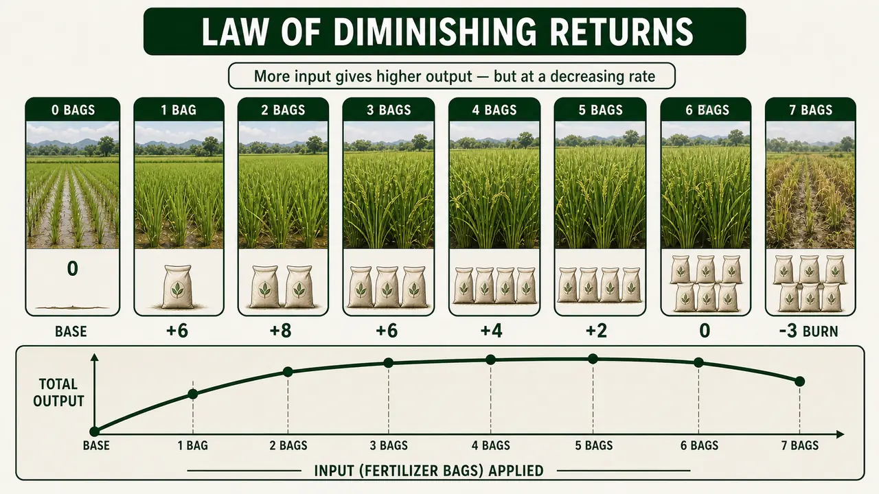
Agricultural Illustration
Consider applying bags of DAP fertilizer to a 1-hectare paddy field:
| Bags of DAP | Total Yield (qtl) | Additional Yield (qtl) | Observation |
|---|---|---|---|
| 0 | 10 | -- | Base yield without fertilizer |
| 1 | 16 | 6 | Sharp increase |
| 2 | 24 | 8 | Increasing returns |
| 3 | 30 | 6 | Diminishing returns begin |
| 4 | 34 | 4 | Returns still declining |
| 5 | 36 | 2 | Very small addition |
| 6 | 36 | 0 | Maximum yield reached |
| 7 | 33 | -3 | Crop burn -- yield falls |
Why Diminishing Returns Operate Earlier in Agriculture
The law applies to both agriculture and industry, but it sets in earlier in agriculture due to greater dependence on natural factors.
| Reason | Explanation | Agricultural Example |
|---|---|---|
| Weather dependence | Farms are open-air systems unlike factories | Drought can nullify extra fertilizer applied |
| Limited mechanization | Many operations still rely on manual or animal power | Transplanting paddy by hand limits scale |
| Limited division of labour | Same worker does multiple seasonal tasks | A farmer must plough, sow, weed, and harvest |
| Land is fixed | Land cannot be manufactured or expanded | India's net sown area has remained nearly constant |
| Soil exhaustion | Continuous cropping depletes fertility | Intensive rice-wheat system in Indo-Gangetic plains |
| Expansion to inferior lands | Rising demand pushes farming to marginal soils | Rainfed farming on rocky Deccan plateau soils |
Limitations of the Law
The law may not operate when:
- Improved cultivation methods are adopted (e.g., precision agriculture, drip irrigation)
- New fertile soils are brought under cultivation (e.g., reclaimed wasteland)
- Insufficient capital has been applied so far (farm is still in the increasing returns phase)
Concepts of Production
Understanding Total Product (TP), Average Product (AP), and Marginal Product (MP) is essential before analysing the production function curve.

Physical Measures
| Measure | Formula | What It Shows | Agricultural Example |
|---|---|---|---|
| Total Physical Product (TPP) | Sum of all output | Cumulative output from all units of input | Total wheat yield from 5 bags of urea = 36 qtl |
| Average Physical Product (APP) | Y / X | Output per unit of input on average | 36 qtl / 5 bags = 7.2 qtl per bag |
| Marginal Physical Product (MPP) | ΔY / ΔX | Additional output from the last unit of input | 5th bag added only 2 qtl |
- TPP indicates the technical efficiency of fixed resources (land, machinery).
- APP indicates the technical efficiency of variable resources (fertilizer, labour).
- MPP is the key measure for decision-making -- it shows the exact contribution of the last unit of input.
Monetary Measures
To compare inputs and outputs in rupee terms, physical products are converted using product price (Py):
| Monetary Measure | Formula | Meaning |
|---|---|---|
| Total Value Product (TVP) | TPP x Py | Total revenue from output |
| Average Value Product (AVP) | APP x Py | Revenue per unit of input |
| Marginal Value Product (MVP) | MPP x Py | Revenue from the last unit of input |
TIP
Profit-maximizing rule: Keep adding input until MVP = MFC (Marginal Factor Cost = price of one unit of input). If MVP > MFC, use more input. If MVP < MFC, you are using too much.
Example: If 1 bag of urea costs Rs 300 (MFC) and the extra wheat it produces sells for Rs 500 (MVP), the farmer should apply that bag. Stop when MVP falls to Rs 300.
Production Function Curve
☘️ NABARD Mains 2020
Table: Relationship between Total, Average and Marginal Products
| Unit of fertilizer X | Total Physical Product (TPP) Y | Average Physical Product APP = TP/X | Marginal Physical Product MPP = ΔTP/ΔX | Remarks |
|---|---|---|---|---|
| 1 | 2 | 2 | 2 | Increasing at increasing rate |
| 2 | 6 | 3 | 4 | Increasing at increasing rate |
| 3 | 12 | 4 | 6 | Increasing at increasing rate |
| 4 | 20 | 5 | 8 | Increasing at increasing rate |
| 5 | 26 | 5.2 | 6 | Increasing at constant or Marginal returns |
| 6 | 30 | 5 | 4 | Increasing at decreasing rate |
| 7 | 33 | 4.7 | 3 | Increasing at decreasing rate |
| 8 | 34 | 4.25 | 1 | Increasing at decreasing rate |
| 9 | 34 | 3.8 | 0 | Increasing at decreasing rate |
| 10 | 33 | 3.3 | -1 | Decreasing or negative marginal |
| 11 | 31 | 2.8 | -2 | Decreasing or negative marginal |
| 12 | 28 | 2.3 | -3 | Decreasing at increasing rate |
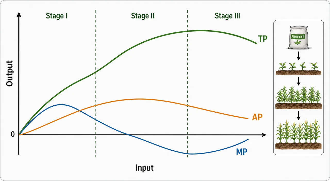
Key Inferences from the Curve
- All TPP, MPP, and APP curves are inverted U-shaped -- they rise, peak, and decline.
- Initially, TPP rises at an increasing rate (curve is concave upward) and MPP is rising.
- At the inflection point (A), MPP reaches its maximum. After this, TPP still rises but at a decreasing rate.
- TPP is maximum at point B where MPP = 0. This is the critical turning point.
Relationship between TP and MP
| When TP is... | MP is... | Agricultural Meaning |
|---|---|---|
| Increasing at increasing rate | Positive and rising | Early fertilizer doses boost yield sharply |
| Increasing at constant rate | Constant | Each dose adds the same yield (rare) |
| Increasing at decreasing rate | Positive but declining | Additional fertilizer helps less and less |
| At maximum | Zero | Crop has reached biological yield potential |
| Decreasing | Negative | Excess fertilizer causes crop burn |
Relationship between MP and AP
| Condition | Effect on AP | Analogy |
|---|---|---|
| MP > AP | AP increases | A student scoring above average raises the class average |
| MP = AP | AP is maximum | Boundary between Stage I and Stage II |
| MP < AP | AP decreases (but stays positive) | A low score pulls down the average |
TIP
Mnemonic -- "MAM": MP crosses AP at Maximum AP. Remember: MP intersects AP from above at AP's peak.
Elasticity of Production (Ep)
Elasticity of production measures the responsiveness of output to changes in input. It is a unit-free ratio useful for comparing across different inputs and crops.
Formula:
Ep = (% change in output) / (% change in input) = (ΔY/ΔX) x (X/Y) = MPP / APP
Ep Values and Their Meaning
| Ep Value | Returns Type | Stage | Agricultural Meaning |
|---|---|---|---|
| Ep > 1 | Increasing returns | Stage I | First 2 irrigations double paddy yield |
| Ep = 1 | Constant returns | End of Stage I | MPP = APP; transition point |
| 0 < Ep < 1 | Diminishing returns | Stage II | Extra fertilizer helps but less each time |
| Ep = 0 | Zero returns | End of Stage II | TPP is maximum; MPP = 0 |
| Ep < 0 | Negative returns | Stage III | Over-irrigation causes waterlogging |
Three Stages of the Production Function
The production function is divided into three stages to identify the rational zone for production decisions.
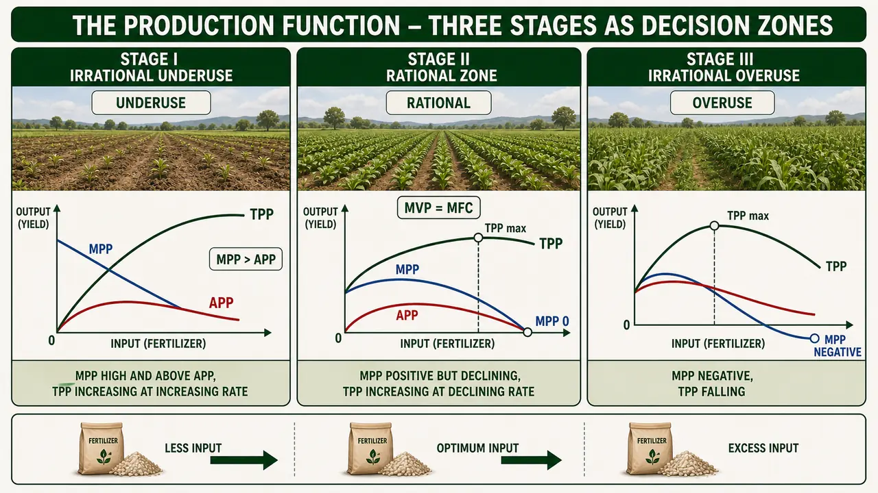
Stage I -- Irrational (Sub-optimal) Zone
WARNING
A rational farmer should never stop in Stage I because input efficiency is still increasing.
| Feature | Detail |
|---|---|
| Starts at | Zero input level (origin) |
| APP | Increasing throughout |
| MPP | Rises to inflection point, then declines but stays above APP |
| TPP | Increasing (first at increasing rate, then decreasing rate) |
| Ep | Greater than 1; equals 1 at the end |
| Ends at | MPP = APP (APP is maximum) |
| MVP vs MFC | MVP > MFC |
| Resource situation | Fixed resources (land) are underutilized |
| Why irrational | Efficiency is still rising -- stopping wastes fixed resources |
Agricultural example: A farmer with 5 acres applies only 1 bag of fertilizer to the entire field. Land is vastly underutilized. Adding more fertilizer will increase both total and average yield.
Stage II -- Rational Zone
IMPORTANT
Stage II is the only rational zone. The profit-maximizing point lies here; its exact location depends on input and output prices.
| Feature | Detail |
|---|---|
| Starts at | APP is maximum (MPP = APP) |
| APP | Decreasing throughout |
| MPP | Positive but declining, always below APP |
| TPP | Increasing at decreasing rate |
| Ep | Between 0 and 1; equals 0 at the end |
| Ends at | MPP = 0 (TPP is maximum) |
| MVP vs MFC | MVP = MFC at the optimum point |
| Resource situation | Variable resources adequate relative to fixed factors |
| Why rational | Both fixed and variable resources are used efficiently |
Agricultural example: A farmer applies 3-5 bags of fertilizer per acre. Each additional bag still increases yield but by a smaller amount. The exact optimum bag depends on fertilizer price and wheat MSP.
Price effect on optimum location within Stage II:
| Scenario | Optimum shifts toward |
|---|---|
| Input price high, output price low | Beginning of Stage II (near max APP) |
| Input price low, output price high | End of Stage II (near max TPP) |
Stage III -- Irrational (Supra-optimal) Zone
WARNING
A rational farmer should never operate here, even if inputs are free, because additional input reduces total output.
| Feature | Detail |
|---|---|
| Starts at | TPP is maximum (MPP = 0) |
| APP | Declining but positive |
| MPP | Negative |
| TPP | Declining at increasing rate |
| Ep | Less than zero |
| MVP vs MFC | MVP < MFC |
| Resource situation | Variable resources in excess |
| Why irrational | More input destroys output |
Agricultural example: Excessive urea causes leaf burn in wheat. Over-irrigation leads to waterlogging in sugarcane. The farmer suffers a double loss:
- Reduced production -- yield falls despite more input
- Wasted cost -- money spent on inputs that harm the crop
Summary: Three Stages at a Glance
| Feature | Stage I (Sub-optimal) | Stage II (Rational) | Stage III (Supra-optimal) |
|---|---|---|---|
| Nature | Irrational | Rational | Irrational |
| APP | Increasing | Decreasing | Decreasing |
| MPP | Positive (rises then falls) | Positive but declining | Negative |
| TPP | Increasing | Increasing (slower) | Decreasing |
| Ep | > 1 | 0 to 1 | < 0 |
| MVP vs MFC | MVP > MFC | MVP = MFC | MVP < MFC |
| Decision | Keep adding input | Find optimum here | Stop -- do not operate |
| Agri example | Under-fertilized field | Optimal fertilizer dose | Crop burn from excess |
TIP
Exam mnemonic -- "SRD":
- Stage I: Sub-optimal (Ep > 1, APP rising)
- Rational: Stage II (0 < Ep < 1, find optimum)
- Dangerous: Stage III (Ep < 0, MPP negative)
Quick recall: "In Stage I, land is wasted. In Stage II, profit is tasted. In Stage III, crops are blasted."
How a Farmer Actually Uses This: The Profit-Maximizing Rule
The theory above translates to one simple farmer decision:
"Stop adding input when the cost of the last unit of input equals the value of the extra output it produces."
Mathematically: MPP × Output Price = Input Price per unit (the optimum point)
Worked Example: Urea on Wheat
| Step | Calculation |
|---|---|
| Price of wheat | ₹2,275/quintal (MSP 2024-25) |
| Price of urea | ₹266/50 kg bag = ₹5.32/kg |
| Question | How much urea should the farmer apply? |
| Rule | Keep applying urea as long as each additional kg produces more than ₹5.32/₹2,275 = 0.0023 quintals (0.23 kg) of extra wheat |
| In practice | Response to urea follows diminishing returns. Early bags give 3-5 qtl extra yield. Later bags give <0.5 qtl. Stop when marginal return ≈ marginal cost |
Stage II is where the farmer should operate — MPP is positive but declining. Stage I means the farmer is under-using inputs (leaving money on the table). Stage III means over-application (wasting money and potentially damaging the crop).
Exam trap: Students confuse "maximum yield" with "maximum profit." Maximum yield occurs at the end of Stage II (MPP = 0), but maximum profit occurs earlier — where MPP × Price = Input Cost. These are different points.
Summary Cheat Sheet
| Concept / Topic | Key Details / Explanation |
|---|---|
| Factor-Product Relationship | How a single variable input transforms into output; all other inputs fixed |
| Central Question | "How much to produce?" — goal is production optimization |
| Also Called | Input-Output Relationship; Fertilizer Response Curve (agronomy) |
| Governing Law | Law of Diminishing Returns (Law of Variable Proportions) |
| Algebraic Form | Y = f(X1 / X2, X3...Xn) — one variable input, rest fixed |
| TPP (Total Physical Product) | Cumulative output from all units of input; indicates efficiency of fixed resources |
| APP (Average Physical Product) | Y / X = output per unit of input; indicates efficiency of variable resources |
| MPP (Marginal Physical Product) | Delta Y / Delta X = additional output from last unit of input; key for decisions |
| MVP (Marginal Value Product) | MPP x Py = revenue from the last unit of input |
| MFC (Marginal Factor Cost) | Price of one unit of input |
| Profit-Maximizing Rule | Keep adding input until MVP = MFC; if MVP > MFC, use more; if MVP < MFC, use less |
| Elasticity of Production (Ep) | MPP / APP = % change in output / % change in input |
| Ep > 1 | Increasing returns (Stage I); MPP > APP |
| 0 < Ep < 1 | Diminishing returns (Stage II); MPP < APP but positive |
| Ep < 0 | Negative returns (Stage III); MPP is negative |
| Stage I (Sub-optimal) | APP increasing, Ep > 1, MVP > MFC; fixed resources underutilized; irrational to stop here |
| Stage II (Rational) | APP decreasing, 0 < Ep < 1, optimum at MVP = MFC; only rational zone |
| Stage III (Supra-optimal) | MPP negative, Ep < 0, TPP declining; never operate here even if inputs are free |
| Stage I ends at | MPP = APP (APP is maximum) |
| Stage II ends at | MPP = 0 (TPP is maximum) |
| MP crosses AP | MP intersects AP from above at AP's peak (MAM mnemonic) |
| Diminishing Returns Earlier in Agriculture | Weather dependence, limited mechanization, land is fixed, soil exhaustion |
| Price Effect on Optimum | High input price / low output price: optimum near start of Stage II. Low input price / high output price: optimum near end of Stage II |
| Mnemonic SRD | Stage I: Sub-optimal, Rational: Stage II, Dangerous: Stage III |