👨🔧 Factor-Factor Relationship: Least Cost Input Combination in Farming
Learn how farmers find the cheapest combination of inputs using isoquants, MRTS, iso-cost lines, and the principle of factor substitution with agricultural examples.
Opening Example
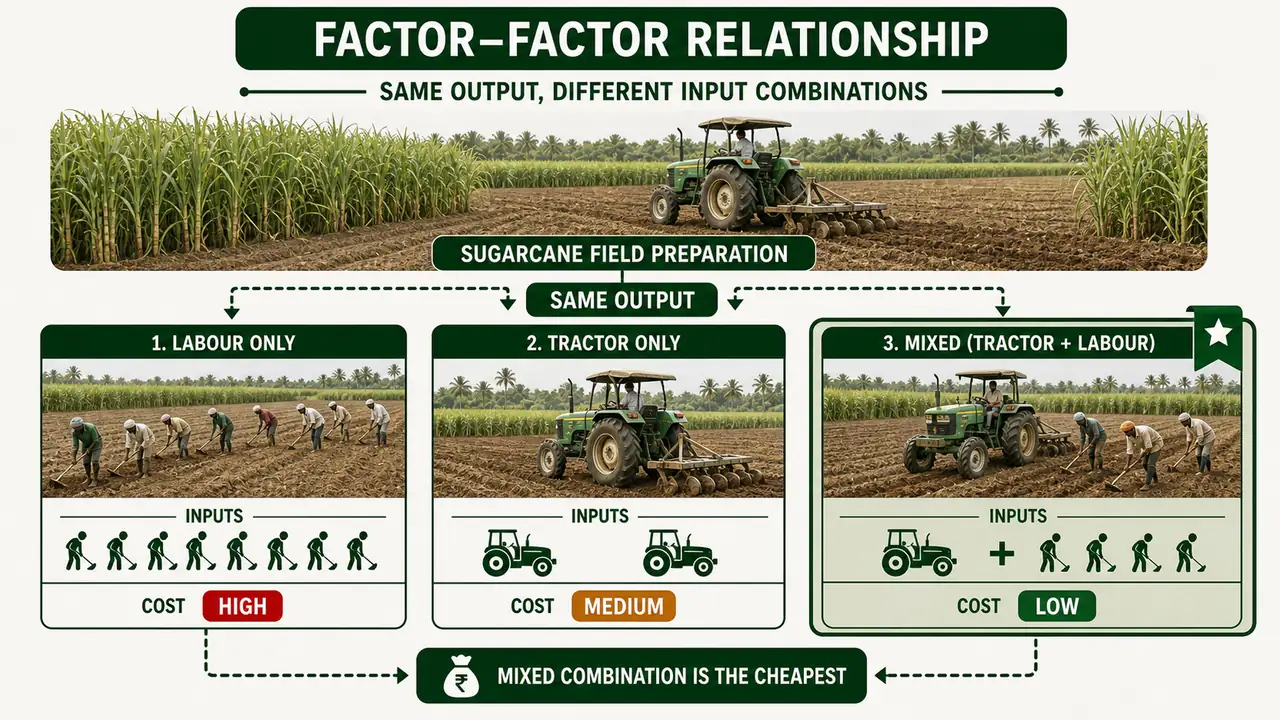
A sugarcane farmer in Maharashtra needs to prepare his field. He can use hired labour or machine (tractor) power -- or a mix of both. Hiring 10 labourers at Rs 400/day costs Rs 4,000. Using a tractor for the full job costs Rs 3,500. But a smart combination -- tractor for primary tillage and labourers for inter-row work -- costs only Rs 2,800 and achieves the same result. Finding this cheapest combination of inputs for a given output is exactly what the Factor-Factor Relationship is about.
What is the Factor-Factor Relationship?
The Factor-Factor Relationship examines how two or more inputs can be combined and substituted to produce a given level of output at the lowest cost.
| Aspect | Detail |
|---|---|
| Also called | Resource Combination / Resource Substitution relationship |
| Central question | "How to produce?" |
| Goal | Cost minimization |
| Output | Kept constant; inputs are varied |
| Choice indicators | Substitution ratio and price ratio |
| Governing principle | Principle of Factor Substitution |
Comparison with Factor-Product Relationship:
Pro Content Locked
Upgrade to Pro to access this lesson and all other premium content.
₹99 charged monthly · Cancel anytime
- All Agriculture & Banking Courses
- AI Lesson Questions (100/day)
- AI Doubt Solver (50/day)
- Glows & Grows Feedback (30/day)
- AI Section Quiz (20/day)
- 22-Language Translation (100/day)
- Recall Questions (20/day)
- AI Quiz (15/day)
- AI Quiz Paper Analysis (100/day)
- AI Step-by-Step Explanations (100/day)
- Spaced Repetition Recall (FSRS)
- AI Tutor
- Immersive Text Questions
- Audio Lessons — Hindi & English
- Mock Tests & Previous Year Papers
- Summary & Mind Maps
- XP, Levels, Leaderboard & Badges
- Generate New Classrooms
- Voice AI Teacher (AgriDots Live)
- AI Revision Assistant
- Knowledge Gap Analysis
- Interactive Revision (LangGraph)
🔒 Secure via Razorpay · Cancel anytime · No hidden fees
Opening Example
A sugarcane farmer in Maharashtra needs to prepare his field. He can use hired labour or machine (tractor) power -- or a mix of both. Hiring 10 labourers at Rs 400/day costs Rs 4,000. Using a tractor for the full job costs Rs 3,500. But a smart combination -- tractor for primary tillage and labourers for inter-row work -- costs only Rs 2,800 and achieves the same result. Finding this cheapest combination of inputs for a given output is exactly what the Factor-Factor Relationship is about.
What is the Factor-Factor Relationship?
The Factor-Factor Relationship examines how two or more inputs can be combined and substituted to produce a given level of output at the lowest cost.
| Aspect | Detail |
|---|---|
| Also called | Resource Combination / Resource Substitution relationship |
| Central question | "How to produce?" |
| Goal | Cost minimization |
| Output | Kept constant; inputs are varied |
| Choice indicators | Substitution ratio and price ratio |
| Governing principle | Principle of Factor Substitution |
Comparison with Factor-Product Relationship:
| Factor-Product | Factor-Factor | |
|---|---|---|
| Question | How much to produce? | How to produce? |
| Variable | One input and output | Two inputs; output fixed |
| Goal | Production optimization | Cost minimization |
Algebraic expression:
Y = f(X1, X2 / X3, X4 ….. Xn)
Output Y is a function of two variable inputs (X1 and X2) while all other inputs are held constant.
Agricultural example: Wheat yield (Y) depends on nitrogen fertilizer (X1) and irrigation water (X2), while land, seed, and labour are fixed.
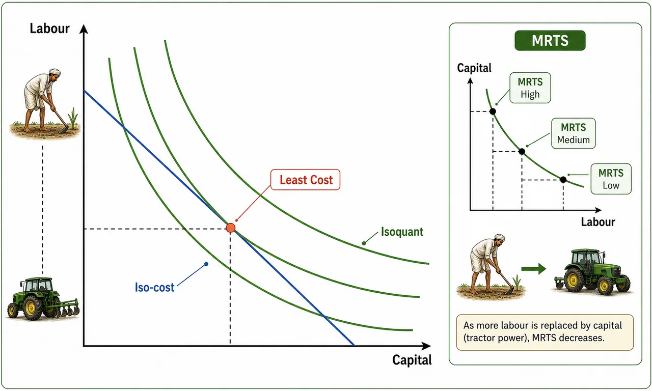
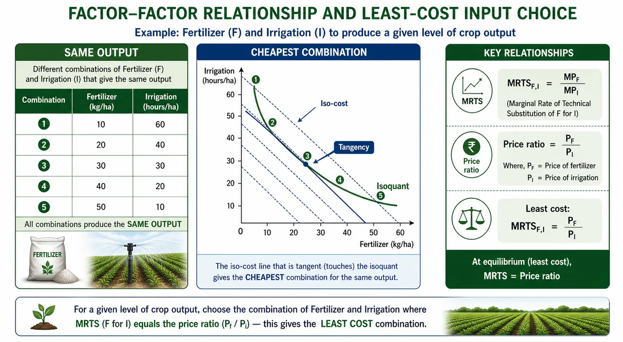
Isoquants (Equal Product Curves)
An isoquant shows all possible combinations of two inputs that produce the same quantity of output. Think of it like a contour line on a map -- a contour connects points of equal elevation; an isoquant connects points of equal output.
An isoquant represents all possible combinations of two resources (X1 and X2) physically capable of producing the same quantity of output.
Other names: Iso-product curve, Equal product curve, Product indifference curve.
Agricultural example: A farmer can produce 40 quintals of paddy using various combinations of fertilizer and irrigation:
| Combination | Fertilizer (kg) | Irrigation (hours) | Output |
|---|---|---|---|
| A | 20 | 80 | 40 qtl |
| B | 40 | 50 | 40 qtl |
| C | 60 | 30 | 40 qtl |
| D | 80 | 20 | 40 qtl |
All four points lie on the same isoquant because they all produce 40 quintals.
Isoquant Map
When multiple isoquants are drawn on one graph, it is called an isoquant map. Each isoquant represents a different output level. Isoquants farther from the origin represent higher output.
Characteristics of Isoquants
IMPORTANT
These five characteristics are frequently asked in exams. Understand the economic reasoning behind each one.
| Characteristic | Reason | Agricultural Analogy |
|---|---|---|
| Slope downward (left to right) | To maintain output, using more of one input means using less of the other | More fertilizer allows less irrigation for the same yield |
| Convex to the origin | Diminishing marginal rate of substitution | Replacing the last unit of irrigation with fertilizer requires increasingly more fertilizer |
| Non-intersecting | Each isoquant = unique output level; intersection would imply same inputs produce two different outputs | One combination of fertilizer + water cannot give both 30 qtl and 40 qtl |
| Higher isoquant = higher output | Isoquants above and to the right use more inputs and produce more | More fertilizer + more water = more paddy |
| Slope = MRTS | The steepness shows the trade-off rate between inputs | Steep slope means large water saving per unit of fertilizer added |
Marginal Rate of Technical Substitution (MRTS)
MRTS measures the amount by which one input is reduced when another input is increased by one unit, keeping output constant. It is the most important concept in factor-factor analysis.
MRTS = (Units of replaced resource) / (Units of added resource)
The slope of the isoquant at any point equals the MRTS at that point.
NOTE
MRTS (input substitution) is analogous to MRPS (output substitution) in the product-product relationship.
Types of Input Relationships
| Type | MRTS | Isoquant Shape | Agricultural Example |
|---|---|---|---|
| Substitutes | Negative (< 0) | Downward sloping | Organic vs inorganic fertilizer |
| Perfect substitutes | Constant negative | Straight line | Family labour vs hired labour |
| Complements | Zero | Cannot substitute | Seed and soil (both needed) |
| Perfect complements | Zero; fixed ratio | L-shaped (right angle) | Tractor and driver; bullock pair and ploughman |
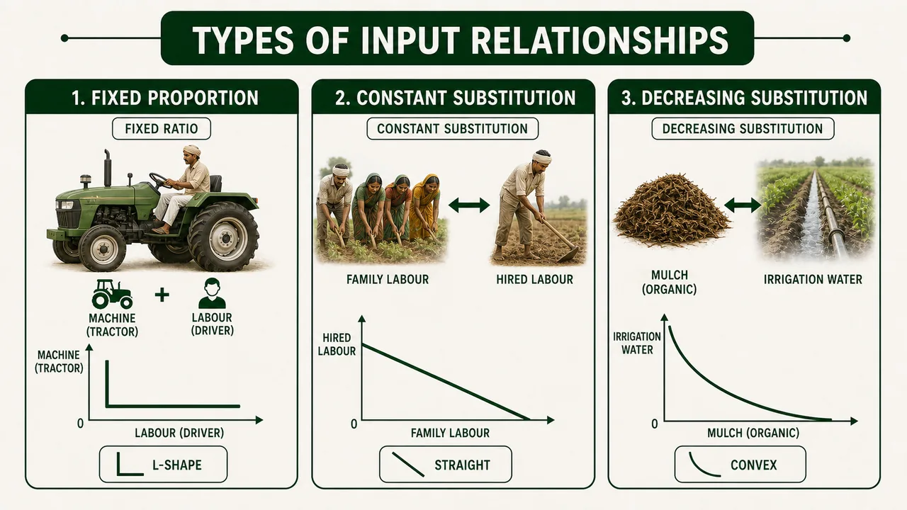
Perfect substitutes: The MRTS remains constant -- you can always swap one for the other at the same rate. The farmer uses whichever is cheaper.
Perfect complements: Only one exact combination works. Extra tractor without a driver is useless; extra driver without a tractor is equally useless.
Three Types of Factor Substitution
The shape of the isoquant depends on how inputs substitute for each other. This is critical for determining the least cost combination.
1. Fixed Proportion (No Substitution)
- Inputs combine in a fixed ratio only.
- Isoquant is L-shaped (right angle).
- Rare in agriculture, but tractor + driver is an approximation.
2. Constant Rate of Substitution
- Each unit of one input replaces a constant quantity of the other.
- Isoquant is a straight line (negatively sloped).
- The MRTS never changes.
Agricultural example: Family labour and hired labour. If 1 family worker always replaces exactly 1 hired worker, the MRTS is constant. The farmer should use only the cheaper labour source -- this leads to an all-or-nothing decision.
3. Decreasing Rate of Substitution (Most Common in Agriculture)
- Each additional unit of one input replaces less and less of the other.
- Isoquant is convex to the origin.
- This is the most realistic pattern in farming.
Agricultural example: Replacing irrigation water with mulch (moisture conservation). The first layer of mulch saves a lot of water. Adding more mulch saves progressively less water because soil moisture retention has biological limits.
| Units of Mulch (X1) | Units of Water (X2) | MRTS (X2 replaced per unit X1) |
|---|---|---|
| 0 | 50 | -- |
| 1 | 42 | 8.0 |
| 2 | 36 | 6.0 |
| 3 | 32 | 4.0 |
| 4 | 30 | 2.0 |
| 5 | 29 | 1.0 |
| X₁ | X₂ | ΔX₁ | ΔX₂ | MRTSX1X2 = ΔX₂/ΔX₁ |
|---|---|---|---|---|
| 1 | 18 | - | - | - |
| 2 | 13 | 1 | 5 | 5/1 = 5 |
| 3 | 9 | 1 | 4 | 4/1 = 4 |
| 4 | 6 | 1 | 3 | 3/1 = 3 |
| 5 | 4 | 1 | 2 | 2/1 = 2 |
Other examples: Capital and labour, concentrates and green fodder, organic and inorganic fertilizers.
TIP
Exam quick recall -- shape tells the story:
| Substitution Type | Isoquant Shape | Decision |
|---|---|---|
| Fixed proportion | L-shaped | Use inputs in fixed ratio |
| Constant rate | Straight line | Use only one input (the cheaper one) |
| Decreasing rate | Convex curve | Use a combination of both inputs |
Iso-cost Line (Budget Line)
The iso-cost line shows all combinations of two inputs that can be purchased with a given budget. It represents the farmer's budget constraint.
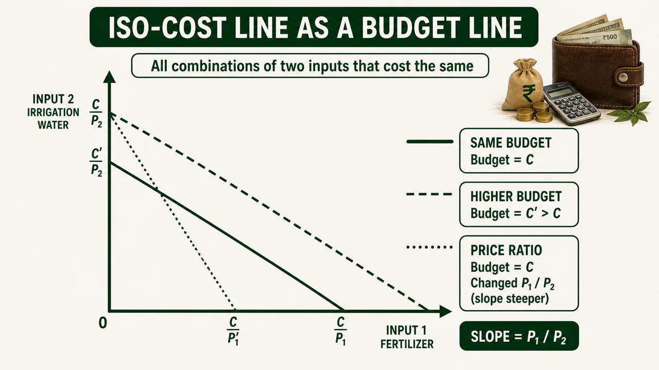
Other names: Price line, Budget line, Iso-outlay line, Factor cost line.
Characteristics
| Property | Explanation | Agricultural Example |
|---|---|---|
| Straight line | Input prices are constant (farmer is a price taker) | Urea price is same whether you buy 1 bag or 10 |
| Moves outward with higher budget | More money = more input combinations possible | Rs 10,000 budget covers more fertilizer + water than Rs 5,000 |
| Slope = price ratio | Slope = PX1 / PX2 | If fertilizer is Rs 6/kg and water Rs 3/hour, slope = 2 |
Finding the Least Cost Combination
The central problem: among all input combinations that produce a target output, which one costs the least?
Three methods can solve this:
Method 1: Simple Arithmetic
Calculate the cost of every possible input combination and pick the cheapest.
Example: Five combinations produce the same wheat yield. With X1 at Rs 3/unit and X2 at Rs 2/unit, the combination of 3 units X1 + 8 units X2 costs Rs 25 -- the least.
Method 2: Algebraic Method
Step 1 -- Compute MRTS:
MRTS = (Units of replaced resource) / (Units of added resource)
Step 2 -- Compute Price Ratio (PR):
PR = (Price per unit of added resource) / (Price per unit of replaced resource)
Step 3 -- Equate MRTS and PR:
IMPORTANT
Key equilibrium condition: MRS = PR
The least cost combination occurs when the rate at which inputs can be technically substituted equals the rate at which they can be exchanged in the market.
Agricultural meaning: If 1 kg extra fertilizer replaces 3 hours of irrigation (MRTS = 3), and fertilizer costs Rs 6/kg while water costs Rs 2/hour (PR = 6/2 = 3), the farmer is at the optimum. If MRTS > PR, use more of the added resource. If MRTS < PR, use less.
Method 3: Graphical Method
Draw the isoquant and iso-cost line on the same graph. The least cost point is where the iso-cost line is tangent to the isoquant.
At the tangency point:
- Slope of isoquant (MRTS) = Slope of iso-cost line (PR)
- No further cost reduction is possible for that output level
- Moving along the isoquant in either direction places the farmer on a higher (more expensive) iso-cost line
Isocline and Expansion Path
Isocline
A line connecting the least cost combinations for all output levels is called an isocline. It passes through all isoquants at points where they have the same slope (same MRTS).
Agricultural example: As a farmer scales up wheat production from 20 to 40 to 60 quintals, the optimal fertilizer-to-water ratio at each level traces out the isocline.
Expansion Path
The most appropriate isocline for a given production period is the expansion path (or scale line). It shows how a rational farmer should adjust the input mix as production scales up or down.
NOTE
Only one expansion path exists at a given set of prices. It is the guide for rational expansion of the farm business.
Ridge Lines (Boundary Lines)
Ridge lines mark the limits of economic substitution on the isoquant map.
| Region | Isoquant Slope | MPP of Both Inputs | Decision |
|---|---|---|---|
| Between ridge lines | Negative | Positive but decreasing | Economically meaningful -- operate here |
| Outside ridge lines | Positive | At least one is negative | Wasteful -- do not operate here |
Agricultural example: Using so much fertilizer that it burns the crop (negative MPP of fertilizer) falls outside the ridge lines. The farmer is wasting money on fertilizer that destroys yield.
How a Farmer Actually Uses This: Least-Cost Input Combination
The farmer's real question: "I need 40 quintals of paddy. Should I spend more on fertilizer or more on irrigation?"
Worked Example: Fertilizer vs Labour for Sugarcane
| Option | Fertilizer Cost | Labour Cost | Total Cost | Output |
|---|---|---|---|---|
| A (more labour) | ₹2,000 | ₹4,000 | ₹6,000 | 80 t/ha |
| B (balanced) | ₹3,000 | ₹2,800 | ₹5,800 | 80 t/ha |
| C (more fertilizer) | ₹4,500 | ₹2,000 | ₹6,500 | 80 t/ha |
Option B is the least-cost combination — same output at lowest total cost. This is the point where the isoquant is tangent to the iso-cost line.
The decision rule: Substitute input X₁ for X₂ as long as the MRTS (rate at which you can swap one input for another while keeping output constant) is greater than the price ratio (P₁/P₂). Stop when MRTS = P₁/P₂.
Analogy: It's like deciding between AC bus and sleeper train for the same journey — different combinations of comfort and cost reach the same destination. You pick the cheapest combination that meets your need.
When input prices change: If labour wages rise (MGNREGA effect), the farmer should substitute toward mechanization. If fertilizer price rises (subsidy reduced), the farmer should substitute toward organic manure + biofertilizer. The optimal mix constantly adjusts to price ratios.
Summary Cheat Sheet
| Concept / Topic | Key Details / Explanation |
|---|---|
| Factor-Factor Relationship | How two inputs are combined and substituted to produce a given output at lowest cost |
| Central Question | "How to produce?" — goal is cost minimization |
| Algebraic Form | Y = f(X1, X2 / X3, X4...Xn) — two variable inputs, others held constant |
| Isoquant | Curve showing all input combos giving the same output; also called iso-product curve or equal product curve |
| Isoquant Map | Multiple isoquants; higher isoquant = higher output |
| Isoquant Properties | Slope downward, convex to origin, non-intersecting, higher = more output, slope = MRTS |
| MRTS | Marginal Rate of Technical Substitution = units of replaced resource / units of added resource |
| Substitutes | MRTS is negative; isoquant slopes downward (e.g., organic vs inorganic fertilizer) |
| Perfect Substitutes | MRTS is constant; isoquant is a straight line (e.g., family labour vs hired labour) |
| Complements | MRTS is zero; cannot substitute one for the other (e.g., seed and soil) |
| Perfect Complements | Fixed ratio only; isoquant is L-shaped (e.g., tractor + driver) |
| Fixed Proportion | L-shaped isoquant; inputs combine in fixed ratio only |
| Constant Rate Substitution | Straight-line isoquant; use only the cheaper input (all-or-nothing decision) |
| Decreasing Rate Substitution | Convex isoquant; most common in agriculture; use a combination of both inputs |
| Iso-cost Line | All input combos purchasable with a given budget; slope = price ratio (Px1/Px2) |
| Least Cost Condition | MRS = PR (Marginal Rate of Substitution = Price Ratio); isoquant tangent to iso-cost line |
| Three Methods | Simple arithmetic, Algebraic (MRTS = PR), Graphical (tangency point) |
| Isocline | Line connecting least cost points across all output levels (same MRTS on each isoquant) |
| Expansion Path | The most appropriate isocline for a given production period; guide for rational farm expansion |
| Ridge Lines | Boundaries of economic substitution; operate only between ridge lines (negative slope, positive MPP) |