🎰 Linear Programming — Optimising Farm Plans with Limited Resources
Understand Linear Programming (LP) for agriculture — definition, assumptions, advantages, limitations, and comparison with budgeting. Includes agricultural examples, shadow prices, exam tips, and summary table for competitive exams.
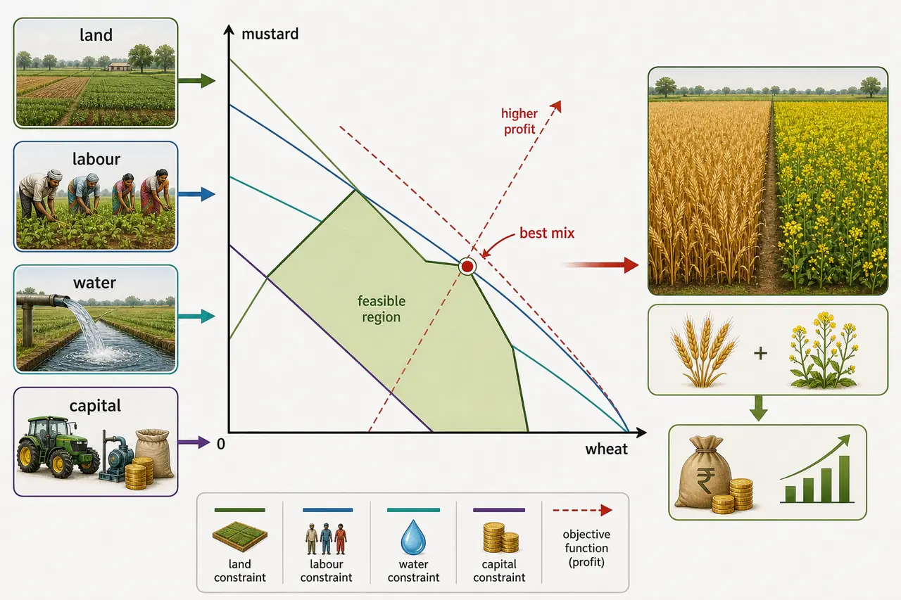
A farmer in Punjab has 10 hectares of land, 500 labour-hours per season, and Rs. 2,00,000 in capital. She can grow wheat (profit Rs. 25,000/ha) or mustard (profit Rs. 18,000/ha), but each crop needs different amounts of labour and capital. What combination of crops will maximise her total profit without exceeding any resource? This is exactly the kind of problem Linear Programming solves.
Linear programming becomes much easier once the learner can see the constraint lines, feasible region, and best decision point together instead of treating them as abstract mathematics.
What Is Linear Programming?
Linear Programming (LP) is a mathematical method for finding the best possible outcome (maximum profit or minimum cost) from a set of linear relationships subject to resource constraints.
- Linear means all relationships between variables are directly proportional — if one hectare of wheat needs 50 kg of fertilizer, two hectares need exactly 100 kg. All relationships plot as straight lines.
- Programming here means planning and scheduling activities to achieve an optimal result — it does not refer to computer coding.
LP was developed by George B. Dantzig in 1947 during the Second World War to solve military logistics problems — allocating limited troops, supplies, and equipment most efficiently. Its use later expanded to agriculture, business, and industry, making it one of the most widely used optimisation techniques in the world.
Pro Content Locked
Upgrade to Pro to access this lesson and all other premium content.
₹99 charged monthly · Cancel anytime
- All Agriculture & Banking Courses
- AI Lesson Questions (100/day)
- AI Doubt Solver (50/day)
- Glows & Grows Feedback (30/day)
- AI Section Quiz (20/day)
- 22-Language Translation (100/day)
- Recall Questions (20/day)
- AI Quiz (15/day)
- AI Quiz Paper Analysis (100/day)
- AI Step-by-Step Explanations (100/day)
- Spaced Repetition Recall (FSRS)
- AI Tutor
- Immersive Text Questions
- Audio Lessons — Hindi & English
- Mock Tests & Previous Year Papers
- Summary & Mind Maps
- XP, Levels, Leaderboard & Badges
- Generate New Classrooms
- Voice AI Teacher (AgriDots Live)
- AI Revision Assistant
- Knowledge Gap Analysis
- Interactive Revision (LangGraph)
🔒 Secure via Razorpay · Cancel anytime · No hidden fees
A farmer in Punjab has 10 hectares of land, 500 labour-hours per season, and Rs. 2,00,000 in capital. She can grow wheat (profit Rs. 25,000/ha) or mustard (profit Rs. 18,000/ha), but each crop needs different amounts of labour and capital. What combination of crops will maximise her total profit without exceeding any resource? This is exactly the kind of problem Linear Programming solves.
Linear programming becomes much easier once the learner can see the constraint lines, feasible region, and best decision point together instead of treating them as abstract mathematics.
What Is Linear Programming?
Linear Programming (LP) is a mathematical method for finding the best possible outcome (maximum profit or minimum cost) from a set of linear relationships subject to resource constraints.
- Linear means all relationships between variables are directly proportional — if one hectare of wheat needs 50 kg of fertilizer, two hectares need exactly 100 kg. All relationships plot as straight lines.
- Programming here means planning and scheduling activities to achieve an optimal result — it does not refer to computer coding.
LP was developed by George B. Dantzig in 1947 during the Second World War to solve military logistics problems — allocating limited troops, supplies, and equipment most efficiently. Its use later expanded to agriculture, business, and industry, making it one of the most widely used optimisation techniques in the world.
Why LP Matters in Agriculture
In farm management, LP helps farmers decide the best combination of crops and livestock given their limited land, labour, water, and capital. It replaces guesswork with a mathematically optimal solution.
LP is used for three types of optimisation problems:
| Optimisation Type | Agricultural Example |
|---|---|
| Maximisation of profit | Best crop mix on a multi-crop farm |
| Minimisation of cost | Cheapest feed ration meeting all nutritional requirements for dairy cattle |
| Minimisation of resource use | Achieving a target yield with least water consumption |
NOTE
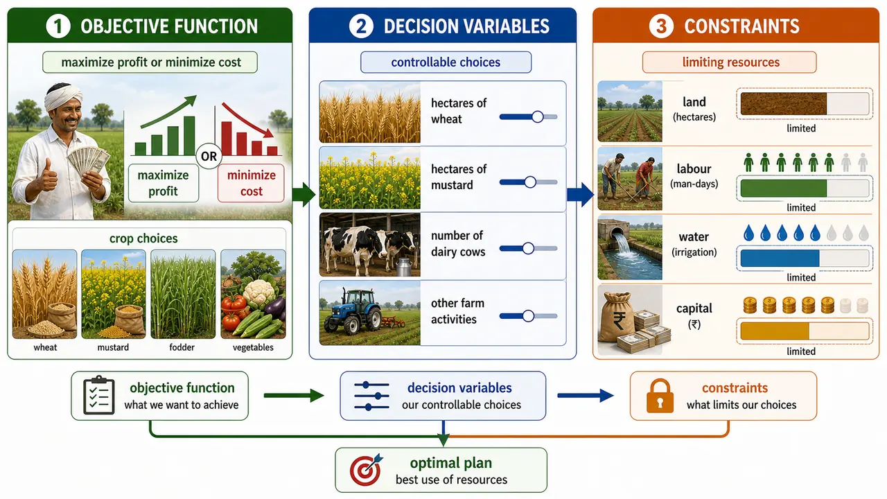
Every LP problem has three essential components: (1) an objective function to be optimised, (2) decision variables representing the activities, and (3) constraints representing resource limitations. Mastering these three components is the key to formulating any LP problem.
Assumptions of Linear Programming
LP solutions are valid only to the extent that these assumptions hold true. Violations can lead to inaccurate results.
| Assumption | What It Means | Agricultural Example |
|---|---|---|
| Linearity | Relationships between inputs and outputs are directly proportional — no economies or diseconomies of scale | If 1 ha of wheat needs 50 kg of fertilizer, then 2 ha need exactly 100 kg |
| Additivity | Total resource use is the simple sum of resources used by each activity — no interaction effects | Growing wheat and rice side by side does not create synergy or interference in the model |
| Divisibility | Resources and outputs can be used in fractional amounts | The model may suggest growing 2.5 ha of paddy — practically rounded to whole numbers |
| Non-negativity | Activity levels and resource use cannot take negative values | You cannot grow negative hectares or use negative labour-hours |
| Finiteness | There is a finite, manageable number of activities and constraints | A farm with 5 crop options and 4 resource constraints |
| Single-value expectations | All prices, yields, and input-output coefficients are known with certainty | Wheat yield is assumed to be exactly 40 q/ha — no weather or market variation |
Exam Tip — Mnemonic: "LADNFS" — Linearity, Additivity, Divisibility, Non-negativity, Finiteness, Single-value expectations. Think: "LAD Never Fails Safely."
Advantages of LP
| Advantage | Explanation | Agricultural Relevance |
|---|---|---|
| Solves allocation problems | Provides a systematic, mathematical approach far more precise than trial-and-error | Allocates scarce water among competing crops on a canal-irrigated farm |
| Gives feasible, practical solutions | The solution satisfies all stated constraints | Crop plan stays within available land, labour, and capital |
| Improves decision quality | Considers all constraints simultaneously, avoiding suboptimal choices | Prevents over-allocating labour to one crop at the expense of another |
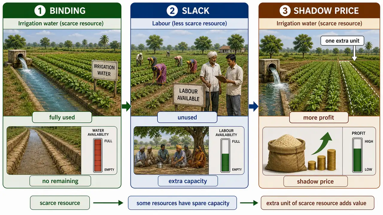
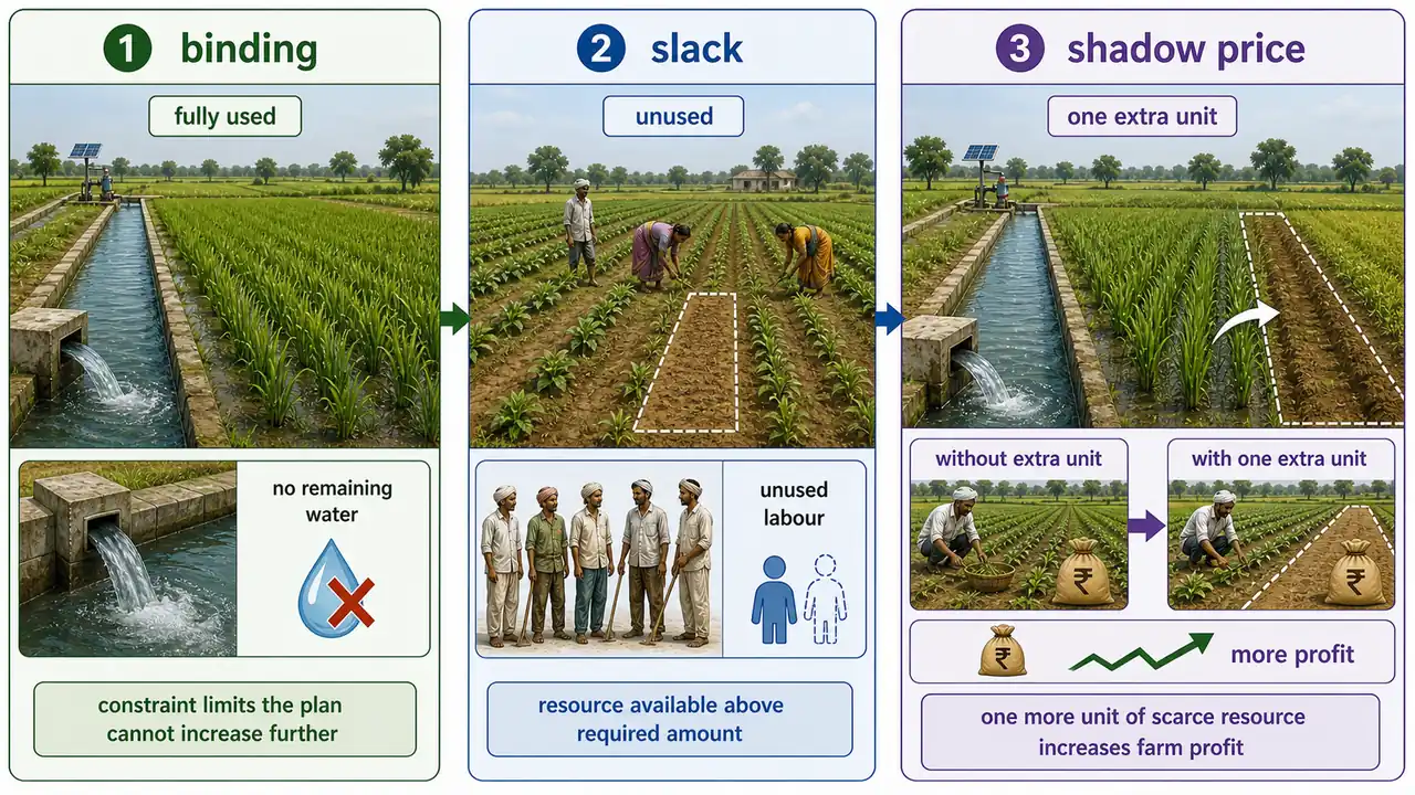
| Identifies binding constraints | Shows which resources are fully used up (binding) and which have slack (unused capacity) | Reveals that water, not land, is the true bottleneck on a farm |
| Ensures optimum resource use | Every unit of every resource is allocated to its most productive use | Each hectare, each labour-hour contributes maximum profit |
| Provides shadow prices (marginal value products) | Tells the farmer how much additional profit one more unit of a scarce resource would generate | A shadow price of Rs. 500 for water means one extra unit of water raises farm profit by Rs. 500 — helping decide whether drilling a bore well is worthwhile |
Limitations of LP
| Limitation | Why It Matters | What to Use Instead |
|---|---|---|
| Linearity assumption | Real agriculture often shows diminishing returns (e.g., more fertilizer eventually adds less yield) — LP cannot capture this | Non-linear programming |
| Single objective only | LP optimises one goal (profit OR cost), but farmers often want to maximise income AND minimise risk AND maintain soil health | Goal programming / Multi-objective programming |
| No time or uncertainty | LP is a static model — it ignores weather risk, price volatility, and changes over time | Dynamic programming / Stochastic programming |
| No guarantee of integer solutions | LP may suggest 3.7 ha of paddy, which is impractical | Integer programming |
| Certainty assumption | Prices, yields, and inputs are assumed known — rarely true in real farming | Sensitivity analysis, parametric programming |
TIP
Despite its limitations, LP remains one of the most powerful tools in farm management. For exams, always mention both advantages and limitations. Remember: LP is best suited for large farms with many enterprises and constraints, where manual budgeting becomes impractical.
LP vs Budgeting — A Key Comparison
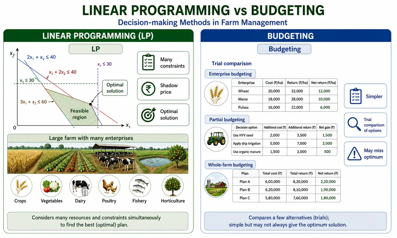
Understanding the difference between LP and budgeting is frequently tested. Budgeting is simpler but may miss the optimal solution. LP guarantees the mathematical optimum but requires more data and computation.
Quick Comparison: LP vs Budgeting
| Feature | Linear Programming | Budgeting |
|---|---|---|
| Approach | Mathematical optimisation | Trial-and-comparison |
| Solution quality | Guaranteed optimal | May not be optimal |
| Complexity handling | Handles many variables and constraints | Best for few variables |
| Assumptions required | Linearity, divisibility, additivity, etc. | Fewer formal assumptions |
| Additional outputs | Shadow prices, slack analysis, sensitivity report | Simple profit estimate only |
| Best suited for | Large farms, many enterprises, many constraints | Small farms, few enterprises, simple changes |
| Agricultural example | Optimising 8-crop plan on a 50-ha irrigated farm | Comparing wheat vs mustard on a 2-ha plot |
Summary Cheat Sheet
| Concept / Topic | Key Details / Explanation |
|---|---|
| Linear Programming (LP) | Mathematical method for finding optimal outcome (max profit or min cost) subject to linear constraints |
| Developed By | George B. Dantzig in 1947 (originally for military logistics) |
| "Linear" | All relationships are directly proportional; plot as straight lines |
| "Programming" | Means planning and scheduling, not computer coding |
| Three LP Components | Objective function (to optimize), decision variables (activities), constraints (resource limits) |
| Three Optimization Types | Maximization of profit, minimization of cost, minimization of resource use |
| Linearity Assumption | Input-output relationships are directly proportional; no economies/diseconomies of scale |
| Additivity | Total resource use = simple sum of resources used by each activity |
| Divisibility | Resources and outputs can be fractional (e.g., 2.5 ha of paddy) |
| Non-negativity | Activity levels and resource use cannot be negative |
| Finiteness | Finite, manageable number of activities and constraints |
| Single-value Expectations | All prices, yields, coefficients assumed known with certainty |
| Assumptions Mnemonic | LADNFS — Linearity, Additivity, Divisibility, Non-negativity, Finiteness, Single-value expectations |
| Shadow Price | Additional profit from one more unit of a scarce resource (e.g., Rs 500 for one extra unit of water) |
| Binding Constraint | A resource that is fully used up — the bottleneck |
| Slack | Unused capacity of a non-binding resource |
| Key Limitation | Cannot handle non-linear relationships, multiple objectives, or uncertainty |
| LP vs Budgeting | LP gives guaranteed optimal solution; budgeting is simpler but may miss optimum |
| LP Best Suited For | Large farms with many enterprises and constraints where manual budgeting is impractical |
| Alternative Methods | Non-linear programming, goal programming, dynamic programming, integer programming |