👨🏻💻 Product-Product Relationship: Optimum Enterprise Combination in Farming
Learn how farmers allocate limited resources among competing enterprises using Production Possibility Curves, MRPS, enterprise relationships, and profit maximization with agricultural examples.
Opening Example
A farmer in Haryana has 10 acres of irrigated land for the rabi season. She can grow wheat, mustard, or a combination of both. If she puts all 10 acres under wheat, she earns Rs 1,80,000. All mustard gives Rs 1,50,000. But allocating 7 acres to wheat and 3 acres to mustard earns Rs 2,00,000 because mustard fetches a premium price and the land suits both crops differently. Deciding the best combination of enterprises with limited resources is the essence of the Product-Product Relationship.
What is the Product-Product Relationship?
The Product-Product Relationship examines how a farmer should allocate fixed resources among two or more competing enterprises to maximize profit.
| Aspect | Detail |
|---|---|
| Also called | Enterprise Relationship |
| Central question | "What to produce?" and "How much of each?" |
| Goal | Profit maximization |
| Inputs | Kept constant; products (outputs) are varied |
| Choice indicators | Substitution ratio (MRPS) and price ratio |
| Governing principles | Principle of Product Substitution; Law of Equi-marginal Returns |
Where it fits among the three fundamental relationships:
Pro Content Locked
Upgrade to Pro to access this lesson and all other premium content.
₹99 charged monthly · Cancel anytime
- All Agriculture & Banking Courses
- AI Lesson Questions (100/day)
- AI Doubt Solver (50/day)
- Glows & Grows Feedback (30/day)
- AI Section Quiz (20/day)
- 22-Language Translation (100/day)
- Recall Questions (20/day)
- AI Quiz (15/day)
- AI Quiz Paper Analysis (100/day)
- AI Step-by-Step Explanations (100/day)
- Spaced Repetition Recall (FSRS)
- AI Tutor
- Immersive Text Questions
- Audio Lessons — Hindi & English
- Mock Tests & Previous Year Papers
- Summary & Mind Maps
- XP, Levels, Leaderboard & Badges
- Generate New Classrooms
- Voice AI Teacher (AgriDots Live)
- AI Revision Assistant
- Knowledge Gap Analysis
- Interactive Revision (LangGraph)
🔒 Secure via Razorpay · Cancel anytime · No hidden fees
Opening Example
A farmer in Haryana has 10 acres of irrigated land for the rabi season. She can grow wheat, mustard, or a combination of both. If she puts all 10 acres under wheat, she earns Rs 1,80,000. All mustard gives Rs 1,50,000. But allocating 7 acres to wheat and 3 acres to mustard earns Rs 2,00,000 because mustard fetches a premium price and the land suits both crops differently. Deciding the best combination of enterprises with limited resources is the essence of the Product-Product Relationship.
What is the Product-Product Relationship?
The Product-Product Relationship examines how a farmer should allocate fixed resources among two or more competing enterprises to maximize profit.
| Aspect | Detail |
|---|---|
| Also called | Enterprise Relationship |
| Central question | "What to produce?" and "How much of each?" |
| Goal | Profit maximization |
| Inputs | Kept constant; products (outputs) are varied |
| Choice indicators | Substitution ratio (MRPS) and price ratio |
| Governing principles | Principle of Product Substitution; Law of Equi-marginal Returns |
Where it fits among the three fundamental relationships:
| Relationship | Question | Goal |
|---|---|---|
| Factor-Product | How much to produce? | Optimize production |
| Factor-Factor | How to produce? | Minimize cost |
| Product-Product | What to produce? | Maximize profit |
Algebraic expression:
Y1 = f (Y2, Y3, ……. Yn)
Output of product Y1 depends on outputs of other products because producing more of one requires diverting resources away from the others.
Agricultural example: On a 10-acre farm, wheat output (Y1) depends on how many acres go to mustard (Y2) and gram (Y3), since total land is fixed.
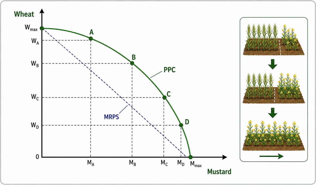
Production Possibility Curve (PPC)
The Production Possibility Curve shows all possible combinations of two products that can be produced with the same total resources. It is the central analytical tool in product-product analysis.
| Other Name | Why It Is Called That |
|---|---|
| Production Possibility Line (PPL) | When the PPC is a straight line |
| Opportunity Curve | Shows all production opportunities with limited resources |
| Iso-resource / Iso-factor Curve | Same total resources used at every point |
| Transformation Curve | Shows the rate at which one product is "transformed" into another |
Agricultural example: A farmer has 5 acres. She can grow cotton (Y1) or maize (Y2):
| Acres for Cotton | Acres for Maize | Cotton (qtl) | Maize (qtl) |
|---|---|---|---|
| 5 | 0 | 30 | 0 |
| 4 | 1 | 27 | 15 |
| 3 | 2 | 22 | 28 |
| 2 | 3 | 16 | 40 |
| 1 | 4 | 9 | 50 |
| 0 | 5 | 0 | 60 |
Plotting these points gives the Production Possibility Curve. Moving along the curve means shifting land (the fixed resource) from one crop to another.
| Allocation of land in acres | Output in Quintals | ||
|---|---|---|---|
| Y₁ | Y₂ | Y₁ | Y₂ |
| 0 | 5 | 0 | 60 |
| 1 | 4 | 8 | 48 |
| 2 | 3 | 15 | 36 |
| 3 | 2 | 21 | 24 |
| 4 | 1 | 26 | 12 |
| 5 | 0 | 30 | 0 |
Types of Enterprise Relationships
Farm enterprises bear several physical relationships to one another. Understanding these is essential for deciding which enterprises to combine.
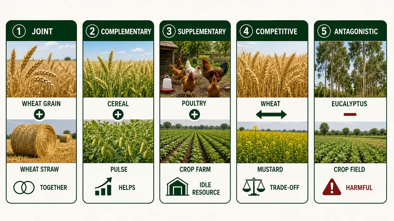
1. Joint Products
Two products produced through a single production process. Production of one (main product) without the other (by-product) is not possible.
| Main Product | Joint Product (By-product) |
|---|---|
| Paddy grain | Paddy straw |
| Wheat grain | Wheat straw (bhusa) |
| Cotton lint | Cotton seed |
| Groundnut kernel | Groundnut haulms |
| Cattle milk | Cattle manure |
| Mustard oil | Mustard cake |
Decision: Always produce together -- they are inseparable.
2. Complementary Relationship
Increasing one product also increases the other. Both enterprises benefit from each other. MRPS is positive (> 0).
Agricultural examples:
- Cereals and pulses in rotation: Pulses fix atmospheric nitrogen, enriching soil for the subsequent cereal crop.
- Crops and livestock: Livestock provides farmyard manure (FYM) that improves soil; crop residues feed the livestock.
- Fish culture in rice paddies: Fish eat insect pests and weeds, reducing crop damage; rice plants provide shade and organic food for fish.
In the figure, complementarity exists from point A to B for Y1 and from C onward for Y2. Within these ranges, increasing one product increases the other.
TIP
Always exploit complementarity first! Produce both complementary products until they enter the competitive range. A wheat-gram rotation benefits both crops before they compete for the same resources.
3. Supplementary Relationship
Increasing or decreasing one product has no effect on the other within a certain range. MRPS is zero.
Agricultural examples:
- A small backyard poultry unit on a crop farm uses kitchen waste, crop residues, and idle family labour without affecting crop production.
- Beekeeping alongside mustard cultivation -- bees use nectar that would otherwise go unused, while pollination boosts mustard yield (this also has a complementary element).
- Mushroom growing in unused farm sheds during the off-season.
A subsidiary enterprise that contributes less than 10% of total farm income is typically supplementary.
Decision: Produce both products up to the point where they become competitive. This uses idle resources productively.
4. Competitive Relationship
Increasing one product decreases the other. They are rivals for the same resources. MRPS is negative (< 0).
This is the most common relationship in agriculture because land, labour, and capital devoted to one crop cannot simultaneously be used for another.
Agricultural examples:
- Wheat vs mustard competing for the same rabi land
- Rice vs maize competing for the same kharif land and irrigation
- Dairy vs poultry competing for the same capital and labour
IMPORTANT
The optimum combination of competitive enterprises is found where MRPS = Price Ratio. This is the equilibrium condition for profit maximization.
5. Antagonistic Products
Two enterprises that are detrimental to each other. Growing both actually harms one or both. Only one should be produced.
Agricultural examples:
- Aquaculture and paddy on adjacent land -- pesticides from paddy harm fish; waterlogging from fish ponds damages paddy
- Eucalyptus plantation near crop fields -- eucalyptus depletes groundwater, harming adjacent crops
- Cotton near tomato -- shared pest (bollworm/fruit borer) multiplies and devastates both
Summary: Enterprise Relationships at a Glance
| Relationship | MRPS | Direction | Decision | Agricultural Example |
|---|---|---|---|---|
| Joint | Fixed | Inseparable | Always produce together | Wheat grain + wheat straw |
| Complementary | Positive (> 0) | Same direction | Produce both up to competitive range | Cereal-pulse rotation |
| Supplementary | Zero | No effect | Produce both -- uses idle resources | Backyard poultry on crop farm |
| Competitive | Negative (< 0) | Opposite direction | Find optimum (MRPS = PR) | Wheat vs mustard for rabi land |
| Antagonistic | Harmful | Detrimental | Produce only one | Aquaculture near paddy |
TIP
Exam mnemonic -- "JCSC-A" (Just Combine, Supplement, Compete, Avoid):
- Joint -- always together
- Complementary -- combine for mutual benefit
- Supplementary -- combine to use idle resources
- Competitive -- find the optimum mix
- Antagonistic -- avoid growing together
Marginal Rate of Product Substitution (MRPS)
MRPS measures the quantity of one product that must be sacrificed to gain one additional unit of another product, with resources held constant. It is the opportunity cost of producing more of one enterprise.
MRPS = (Units of replaced product) / (Units of added product)
Agricultural example: If shifting 1 acre from wheat to mustard reduces wheat by 3 quintals but increases mustard by 5 quintals, the MRPS of mustard for wheat = 3/5 = 0.6. Each quintal of mustard gained costs 0.6 quintals of wheat.
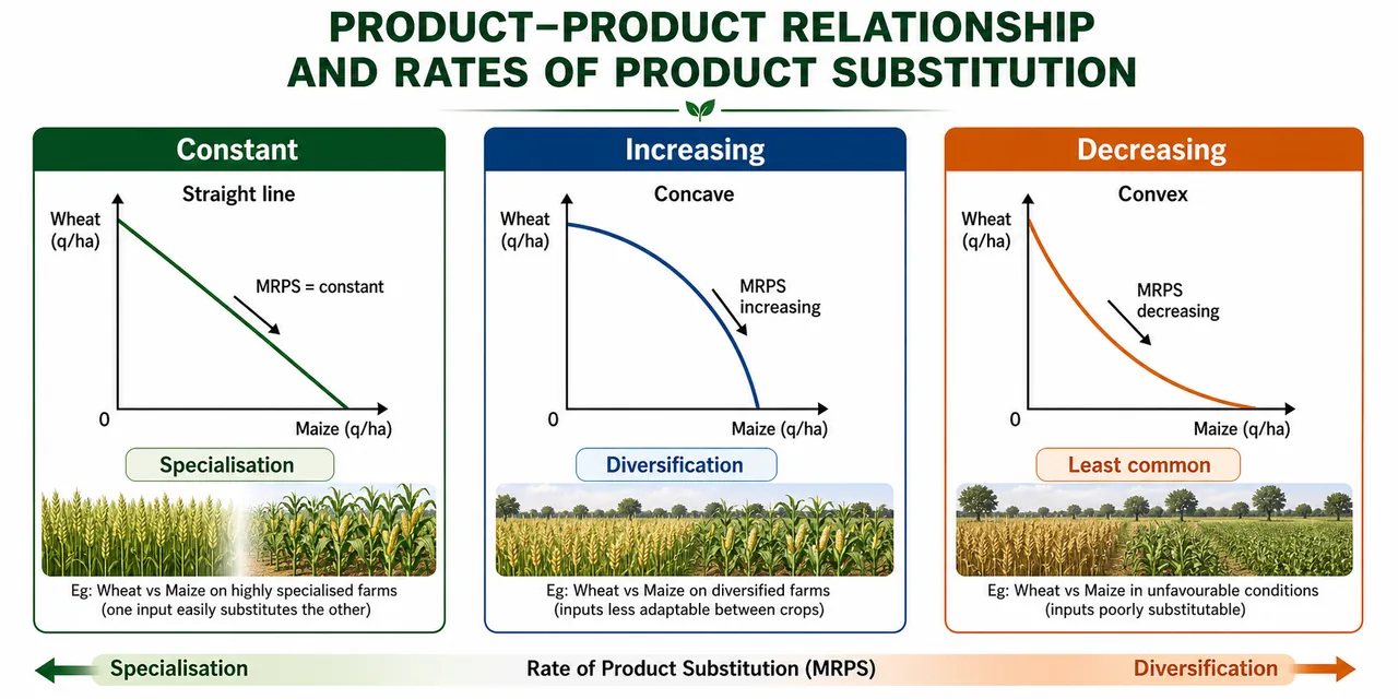
Types of Product Substitution
When two products are competitive, they substitute at one of three rates. The type determines the shape of the PPC and the farmer's strategy.
1. Constant Rate of Product Substitution (CRPS)
- Each unit increase in one product sacrifices a constant quantity of the other.
- PPC is a straight line (negatively sloped).
- Leads to specialization -- produce only the more profitable product.
Agricultural example: Gram and wheat substituting for land at a constant rate. If every acre shifted from wheat to gram always sacrifices 4 quintals of wheat and gains 3 quintals of gram, the MRPS is constant at 4/3.
| Y₁ | ΔY₂ | ΔY₁ | ΔY₂ | MRS |
|---|---|---|---|---|
| 0 | 40 | - | - | - |
| 10 | 30 | 10 | 10 | 10/10 = 1 |
| 20 | 20 | 10 | 10 | 10/10 = 1 |
| 30 | 10 | 10 | 10 | 10/10 = 1 |
| 40 | 0 | 10 | 10 | 10/10 = 1 |
Decision: With constant substitution, grow whichever crop has the higher price relative to MRPS. This is an all-or-nothing choice.
2. Increasing Rate of Product Substitution (IRPS) -- Most Common in Agriculture
- Each unit increase in one product requires larger and larger sacrifice of the other.
- PPC is concave to the origin.
- Leads to diversification -- produce a combination of both products.
This is the most common type in agriculture because land is not homogeneous. The first acres shifted are the most suitable; subsequent acres are progressively less productive in the new use.
Agricultural example: Rice vs maize on 10 acres. The first 2 acres shifted from rice to maize are high-ground plots ideal for maize, sacrificing little rice. But the last 2 acres are low-lying paddy land poorly suited for maize, requiring large rice sacrifice for small maize gain.
| Acre Shifted | Rice Lost (qtl) | Maize Gained (qtl) | MRPS |
|---|---|---|---|
| 1st | 2 | 5 | 0.4 |
| 2nd | 3 | 4 | 0.75 |
| 3rd | 5 | 3 | 1.67 |
| 4th | 8 | 2 | 4.0 |
The MRPS increases -- each additional unit of maize costs more and more rice.
| Y₁ | ΔY₂ | ΔY₁ | ΔY₂ | MRS |
|---|---|---|---|---|
| 0 | 60 | - | - | - |
| 8 | 48 | 8 | 12 | 1.50 |
| 15 | 36 | 7 | 12 | 1.72 |
| 21 | 24 | 6 | 12 | 2 |
| 26 | 12 | 5 | 12 | 2.40 |
| 30 | 0 | 4 | 12 | 3 |
TIP
Key exam point: Increasing rate of product substitution (concave PPC) is the most common type in agriculture and leads to diversification. Constant rate (linear PPC) leads to specialization. This explains why most Indian farms grow multiple crops.
3. Decreasing Rate of Product Substitution (DRPS)
- Each unit increase in one product requires less and less sacrifice of the other.
- PPC is convex to the origin.
- Occurs under conditions of increasing returns. Least common in agriculture.
| Y₁ | Y₂ | ΔY₁ | ΔY₂ | MRS |
|---|---|---|---|---|
| 1 | 18 | - | - | - |
| 2 | 13 | 1 | 5 | 5 |
| 3 | 9 | 1 | 4 | 4 |
| 4 | 6 | 1 | 3 | 3 |
| 5 | 4 | 1 | 2 | 2 |
Comparison of Substitution Types
| Type | PPC Shape | MRPS Pattern | Strategy | Commonality |
|---|---|---|---|---|
| Constant | Straight line | Unchanged | Specialization | Rare |
| Increasing | Concave | Rising | Diversification | Most common |
| Decreasing | Convex | Falling | Extreme specialization | Least common |
Iso-Revenue Line (Iso-Income Line)
The iso-revenue line shows all combinations of two products that yield the same total revenue. It is to product-product analysis what the iso-cost line is to factor-factor analysis.
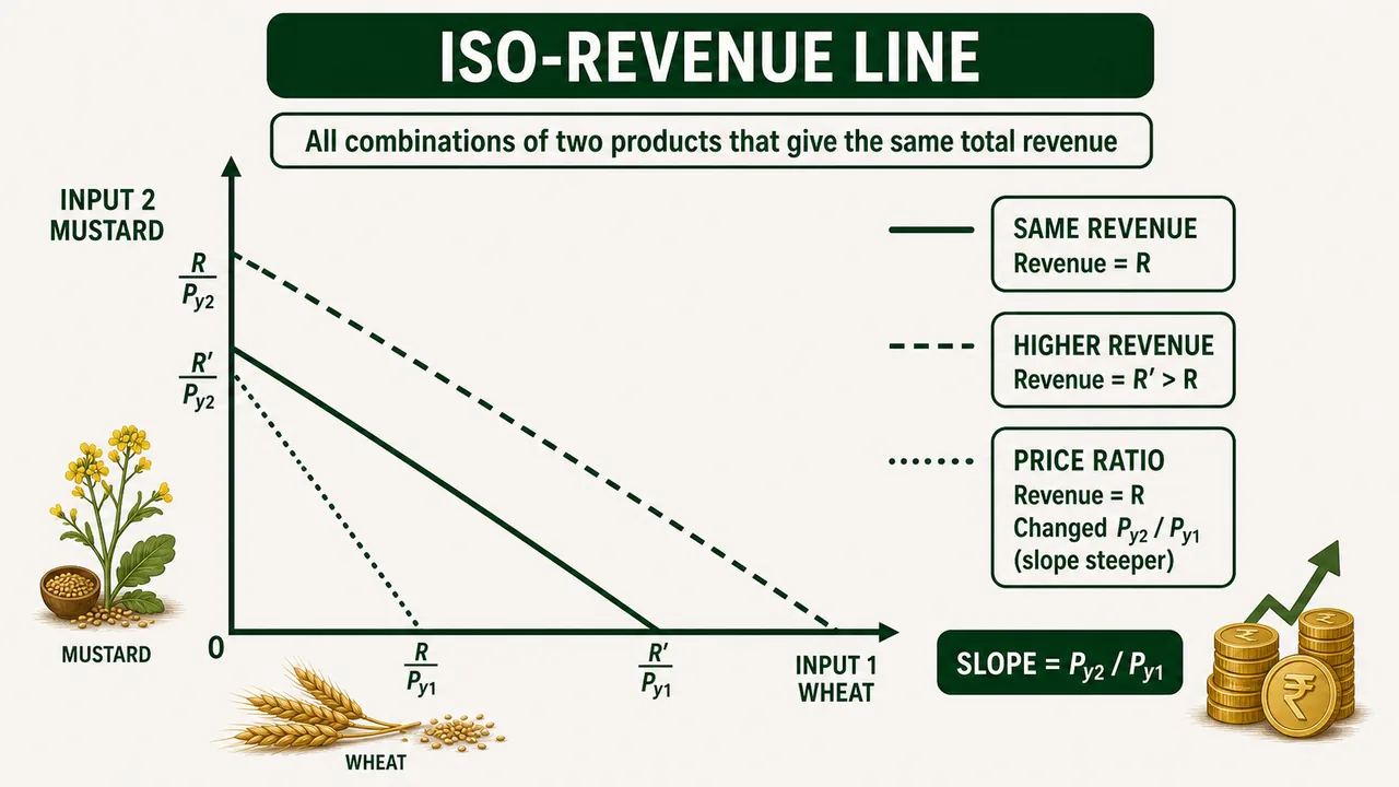
Other names: Iso-return line, Iso-income line.
Characteristics
| Property | Explanation | Agricultural Example |
|---|---|---|
| Straight line | Product prices are constant (farmer is a price taker) | Wheat MSP is the same whether the farmer sells 10 or 100 quintals |
| Moves outward with higher revenue | Higher revenue target = farther from origin | Rs 2,00,000 revenue line is farther out than Rs 1,50,000 |
| Slope = output price ratio | Slope = PY2 / PY1 | If wheat = Rs 2,000/qtl and mustard = Rs 5,000/qtl, slope = 5000/2000 = 2.5 |
Finding the Optimum Product Combination
Three methods determine the enterprise mix that maximizes revenue from fixed resources.
Method 1: Tabular Method
Calculate total revenue for every possible product combination. Choose the one with the highest revenue.
PY1 = Rs 7/kg; PY2 = Rs 10/kg
| S. No. | y₁ (kg) | y₂ (kg) | Py₁.y₁ + Py₂.y₂ = Total Income in Rupees |
|---|---|---|---|
| 1 | 0 | 78 | 0 + 78 = 780 |
| 2 | 10 | 76 | 70 + 760 = 830 |
| 3 | 20 | 72 | 140 + 720 = 860 |
| 4 | 30 | 67 | 210 + 670 = 880 |
| 5 | 40 | 61 | 280 + 610 = 890 |
| 6 | 50 | 48 | 350 + 480 = 830 |
| 7 | 60 | 28 | 420 + 280 = 700 |
| 8 | 70 | 0 | 490 + 0 = 490 |
The 5th combination gives the highest return -- this is the optimum.
Method 2: Algebraic Method
Step 1 -- Compute MRPS:
MRPS = (Units of replaced product) / (Units of added product)
Step 2 -- Compute Price Ratio (PR):
PR = (Price per unit of added product) / (Price per unit of replaced product)
Step 3 -- Equate MRPS and PR:
IMPORTANT
Equilibrium condition: MRPS = PR
The optimum enterprise combination occurs when the rate at which products can be technically substituted equals the rate at which they can be exchanged in the market.
Method 3: Graphical Method
Draw the PPC and iso-revenue line on the same graph. The optimum is where the iso-revenue line is tangent to the PPC.
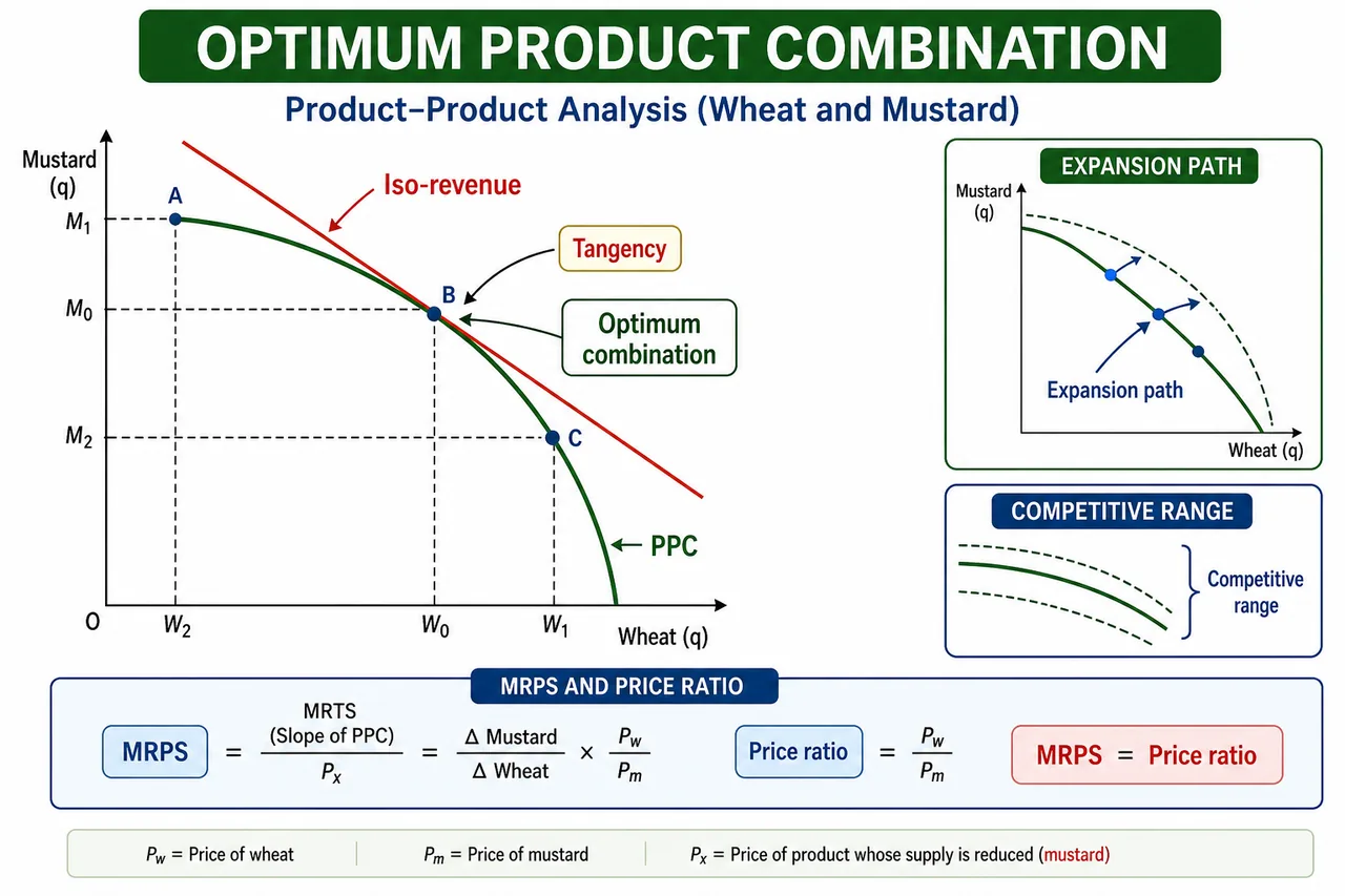
At tangency point C:
- Slope of PPC (MRPS) = Slope of iso-revenue line (PR)
- This is the maximum revenue point
- Note the contrast with factor-factor analysis: there we seek the iso-cost line closest to the origin (minimize cost); here we seek the iso-revenue line farthest from the origin (maximize revenue)
Expansion Path
The locus of tangency points across different PPCs forms the expansion path. It shows the most profitable enterprise combination at each resource level.
Ridge Lines in Product-Product Analysis
Ridge lines separate the competitive range (economically meaningful) from the complementary range on the PPC.
| Region | PPC Slope | MRPS | Enterprise Relationship |
|---|---|---|---|
| Within ridge lines | Negative | < 0 | Competitive — operate here |
| On ridge lines | Zero | 0 | Supplementary — boundary |
| Outside ridge lines | Positive | > 0 | Complementary — exploit first |
Agricultural example: Within ridge lines, shifting 1 acre from wheat to mustard reduces wheat and increases mustard (competitive). Outside ridge lines, both can increase (complementary -- as in a rotation benefit). The farmer should first exploit complementarity, then optimize within the competitive range.
Price-Based Decision Rules
When the price of a product changes, the farmer adjusts the enterprise mix:
| Condition | Meaning | Decision |
|---|---|---|
| ΔY₁ · P_Y₁ > ΔY₂ · P_Y₂ | Extra revenue from Y₁ exceeds Y₂ | Shift resources toward Y₁ |
| ΔY₁ · P_Y₁ < ΔY₂ · P_Y₂ | Extra revenue from Y₂ exceeds Y₁ | Shift resources toward Y₂ |
| ΔY₁ · P_Y₁ = ΔY₂ · P_Y₂ | Both equally profitable | Equilibrium — MRPS = PR |
Agricultural example: If wheat MSP rises from Rs 2,000 to Rs 2,275/qtl while mustard remains at Rs 5,050/qtl, the farmer should allocate more land to wheat until the marginal revenue from the last acre of wheat equals that from the last acre of mustard.
Master Summary Table: Three Fundamental Relationships
| Feature | Factor-Product | Factor-Factor | Product-Product |
|---|---|---|---|
| Question | How much to produce? | How to produce? | What to produce? |
| Goal | Production optimization | Cost minimization | Profit maximization |
| Variable | One input + output | Two inputs; output fixed | Two outputs; input fixed |
| Governing law | Diminishing Returns | Factor Substitution | Product Substitution |
| Key curve | Production Function | Isoquant | PPC |
| Budget/Revenue line | -- | Iso-cost line | Iso-revenue line |
| Equilibrium | MVP = MFC | MRS = PR | MRPS = PR |
| Choice indicator | Price ratio (Px/Py) | Substitution + price ratio | Substitution + price ratio |
TIP
Exam mnemonic -- "HHW" for the three questions:
- Factor-Product: How much?
- Factor-Factor: How?
- Product-Product: What?
Memory aid: "The farmer first asks WHAT to grow (product-product), then HOW to grow it (factor-factor), then HOW MUCH input to use (factor-product)."
How a Farmer Actually Uses This: Crop Allocation Decision
The farmer's real question: "I have 5 acres. How much land should I give to wheat vs mustard?"
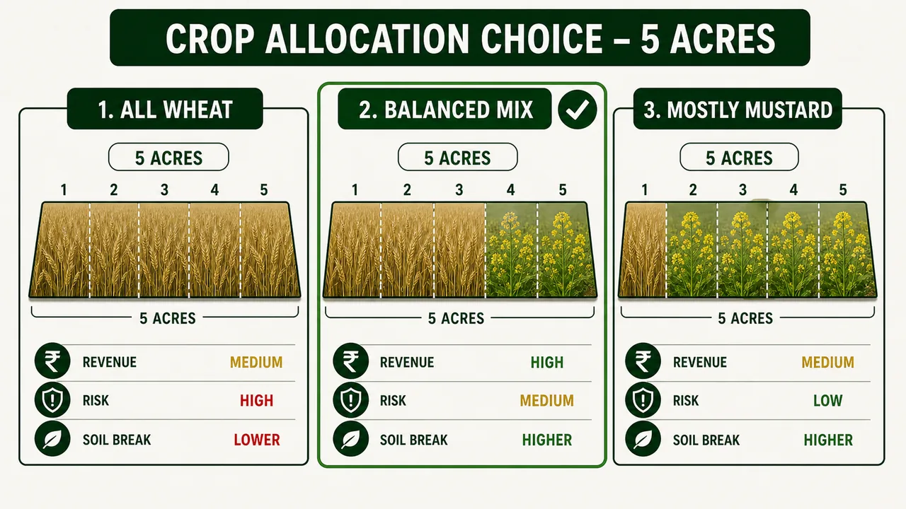
Worked Example: Wheat vs Mustard (Rabi, North India)
| Allocation | Wheat (acres) | Mustard (acres) | Wheat Revenue (@ ₹2,275/qtl, 50 qtl/ha yield) | Mustard Revenue (@ ₹5,650/qtl, 18 qtl/ha yield) | Total Revenue |
|---|---|---|---|---|---|
| All wheat | 5 | 0 | ₹2,80,000 | ₹0 | ₹2,80,000 |
| Mostly wheat | 4 | 1 | ₹2,24,000 | ₹25,000 | ₹2,49,000 |
| Balanced | 3 | 2 | ₹1,68,000 | ₹50,000 | ₹2,18,000 |
| Mostly mustard | 1 | 4 | ₹56,000 | ₹1,00,000 | ₹1,56,000 |
In this example, all-wheat gives highest revenue. But the farmer must also consider:
- Risk diversification — if wheat price crashes or disease hits, mustard provides insurance
- Soil health — mustard (Cruciferae) breaks cereal disease cycle
- Input costs — mustard needs less fertilizer and irrigation than wheat
- Bee income — mustard enables honey production as a bonus enterprise
The decision rule: Allocate land so that the MRPS (extra revenue from shifting one more acre to crop A ÷ lost revenue from crop B) equals the price ratio of the two crops. In practice, most farmers diversify for risk management rather than pure profit maximization.
How prices change the decision: If government raises mustard MSP significantly (as happened in recent years), farmers shift land from wheat to mustard. This is the PPC in action — the same fixed resource (land) being reallocated based on relative prices.
Summary Cheat Sheet
| Concept / Topic | Key Details / Explanation |
|---|---|
| Product-Product Relationship | How to allocate fixed resources among competing enterprises to maximize profit |
| Central Question | "What to produce?" and "How much of each?" — goal is profit maximization |
| Algebraic Form | Y1 = f(Y2, Y3...Yn) — output of one product depends on outputs of others (shared resources) |
| Production Possibility Curve (PPC) | All possible combinations of two products from the same total resources |
| PPC Other Names | Opportunity Curve, Iso-resource Curve, Transformation Curve |
| Joint Products | Produced through a single process; inseparable (e.g., wheat grain + wheat straw, cotton lint + cottonseed) |
| Complementary Relationship | Increasing one product also increases the other; MRPS is positive (> 0) (e.g., cereal-pulse rotation) |
| Supplementary Relationship | One product has no effect on the other; MRPS is zero; uses idle resources (e.g., backyard poultry) |
| Competitive Relationship | Increasing one decreases the other; MRPS is negative (< 0); most common in agriculture |
| Antagonistic Products | Enterprises that are detrimental to each other; produce only one (e.g., eucalyptus near crops) |
| Subsidiary Enterprise Rule | Contributes less than 10% of total farm income = typically supplementary |
| MRPS | Marginal Rate of Product Substitution = units of replaced product / units of added product |
| Constant Rate (CRPS) | PPC is a straight line; leads to specialization (all-or-nothing choice) |
| Increasing Rate (IRPS) | PPC is concave to origin; MRPS rising; leads to diversification; most common in agriculture |
| Decreasing Rate (DRPS) | PPC is convex to origin; MRPS falling; least common in agriculture |
| Iso-Revenue Line | All product combos giving the same total revenue; slope = output price ratio (Py2/Py1) |
| Optimum Condition | MRPS = Price Ratio — where iso-revenue line is tangent to PPC |
| Three Methods | Tabular (calculate all revenues), Algebraic (MRPS = PR), Graphical (tangency point) |
| Ridge Lines | Separate competitive range (negative MRPS) from complementary range (positive MRPS) |
| Expansion Path | Locus of tangency points across different PPCs; most profitable enterprise combo at each resource level |
| Three Relationships | Factor-Product: How much? Factor-Factor: How? Product-Product: What? Equilibria: MVP=MFC, MRS=PR, MRPS=PR |
| JCSC-A Mnemonic | Joint (together), Complementary (combine), Supplementary (use idle resources), Competitive (optimize), Antagonistic (avoid) |