🙅🏼‍♂️Returns to Scale in Agriculture

Opening Example

Imagine a farmer cultivates 2 hectares of wheat using 1 worker, 50 kg seed, and 25 kg fertilizer and harvests 20 quintals. Now suppose he doubles everything — 4 hectares, 2 workers, 100 kg seed, 50 kg fertilizer. If his harvest jumps to 50 quintals (more than double), he is experiencing increasing returns to scale. This concept of changing all inputs together in the same proportion and observing the effect on output is what Returns to Scale is all about.

---

What Are Returns to Scale?

Returns to scale describe the behaviour of output when all inputs are increased or decreased simultaneously in the same proportion. The proportion among inputs remains unchanged — only the scale of operation changes.

Unlike the Law of Variable Proportions (where only one input varies and others stay fixed), returns to scale examines what happens when the entire scale of the farm changes.

---

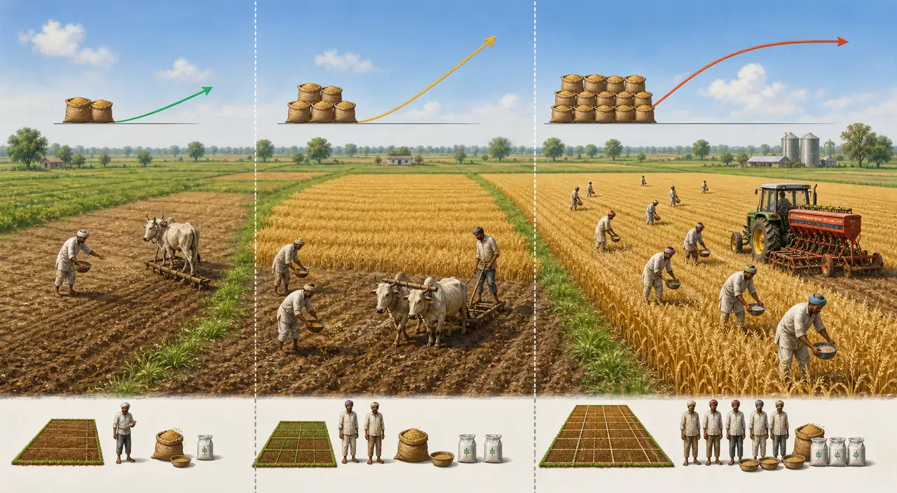
Three Stages of Returns to Scale

When all inputs are increased in the same proportion, output passes through three distinct stages:

Stage	Name	Output Behaviour	Agricultural Reason
I	Increasing Returns to Scale	Output rises more than proportionally	Better division of labour, efficient use of machinery, bulk purchase of seeds and fertilizers
II	Constant Returns to Scale	Output rises exactly in proportion	Farm operates at its most balanced and optimal scale
III	Diminishing Returns to Scale	Output rises less than proportionally	Management difficulties, coordination problems, supervision lapses over large areas

---

Numerical Example

Consider a wheat farm where land and labour are increased together:

Scale	Land (acres)	Workers	Total Product (quintals)	Marginal Product (quintals)	Stage
1x	3	1	2	—	—
2x	6	2	5	3	Increasing
3x	9	3	9	4	Increasing
4x	12	4	12	3	Constant
5x	15	5	14	2	Diminishing

• From scale 1x to 2x, output more than doubles (2 to 5) — increasing returns.
• From scale 3x to 4x, output increases by exactly 3 — constant returns.
• Beyond 4x, each additional unit of scale adds less output — diminishing returns set in because managing 15+ acres with proportionally more workers becomes harder.

Scale of Inputs	Total Physical Product in Quintals	Marginal Physical Product in Quintals	Remarks
1 acres + 3 workers	2	2	Increasing Return
2 acres + 6 workers	5	3	Increasing Return
3 acres + 9 workers	9	4	Increasing Return
4 acres + 12 workers	14	5	Increasing Return
5 acres + 15 workers	19	5	Constant Return
6 acres + 18 workers	24	5	Constant Return
7 acres + 21 workers	28	4	Decreasing Return
8 acres + 24 workers	31	3	Decreasing Return
9 acres + 27 workers	33	2	Decreasing Return

Exam Tip: In practice, the Law of Variable Proportions is more commonly applicable than returns to scale because it is nearly impossible to increase all inputs in exactly the same proportion on a real farm.

---

Summary of Basic Production Relationships

---

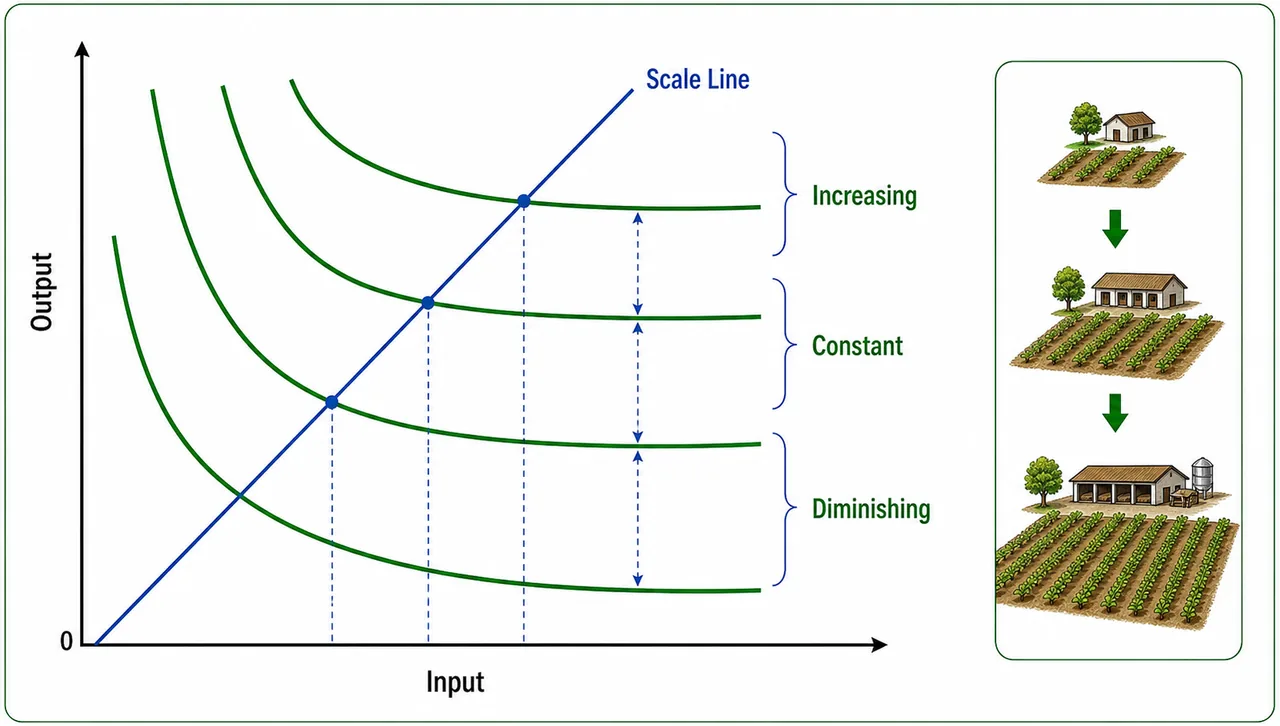
Isoquant Analysis of Returns to Scale

Returns to scale can also be understood using the scale line (a ray from the origin) on an isoquant map. The distance between successive isoquants along the scale line reveals the type of returns:

Type	Distance Between Isoquants (AB, BC, CD)	Meaning
Increasing returns	AB > BC > CD (distances shrink)	Less additional input needed for each successive output increase
Constant returns	AB = BC = CD (distances equal)	Same additional input yields same additional output
Diminishing returns	AB < BC < CD (distances widen)	More additional input needed for same output increment

Agricultural example: A mango orchard doubles all inputs (land, saplings, labour, water). Initially, the orchard benefits from better pollination and efficient irrigation layout (increasing returns). At optimal scale, returns are constant. Beyond that, pest management and supervision become difficult (diminishing returns).

---

Law of Variable Proportions vs. Returns to Scale

Feature	Law of Variable Proportions	Returns to Scale
Inputs changed	Only one input varies; others fixed	All inputs change simultaneously
Proportion	Input proportions change	Input proportions remain same
Time period	Short-run concept	Long-run concept
Practical relevance	Highly relevant to everyday farming	More of theoretical interest
Example	Adding more fertilizer to a fixed plot of paddy	Doubling the entire paddy farm — land, seed, fertilizer, labour
Stages	Increasing, Diminishing, Negative MPP	Increasing, Constant, Diminishing

Law of Variable Proportion	Returns to Scale
Describes the change in output when a single input is varied.	Returns to the change in output when all inputs are varied in equal proportion.
At least one factor is kept constant or fixed.	All factors are varied.
Input proportions among factors remains the same.	Input proportions among factors remains the same.
Short run production function.	Long run production function.
Output includes stages: increasing, decreasing returns.	Output includes stages: increasing, constant, decreasing.
Increasing returns are due to better use of fixed factor.	Increasing returns are due to economies of scale.
Maximum output is due to optimum use of fixed factors.	Maximum output is due to optimum combination of all factors.
Diminishing returns are due to inefficiency arising out of over utilization of fixed factor.	Diminishing returns are due to diseconomies of scale.
Internal dis economies of scale.	Internal dis economies of scale.

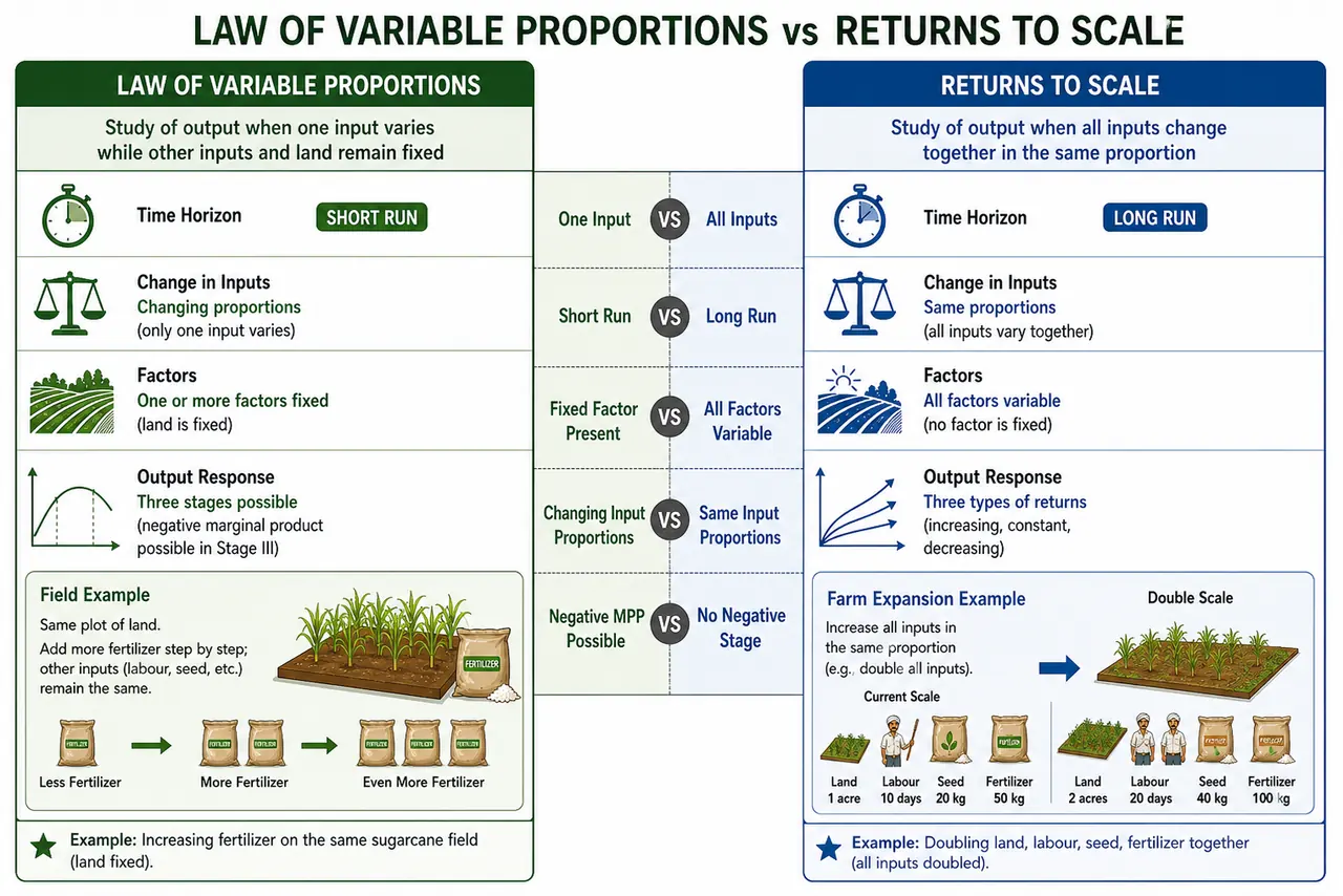
Mnemonic — “VO-SL”:

• Variable proportions = One input changes (short-run)
• Scale = aLl inputs change (long-run)

---

Summary Table

Concept	Key Point
Returns to Scale	Effect on output when all inputs change in the same proportion
Increasing Returns	Output grows faster than inputs — economies of scale (e.g., better machinery use on larger farms)
Constant Returns	Output grows at the same rate as inputs — optimal scale
Diminishing Returns	Output grows slower than inputs — diseconomies of scale (management, supervision)
Isoquant test	Shrinking distance = increasing; equal = constant; widening = diminishing
Practical note	Law of Variable Proportions is more relevant in real farming than returns to scale

Summary Cheat Sheet

Concept / Topic	Key Details / Explanation
Returns to Scale	Effect on output when all inputs are changed simultaneously in the same proportion
Key Difference from Variable Proportions	Returns to scale: all inputs change (long-run). Variable Proportions: one input changes (short-run)
Increasing Returns to Scale	Output rises more than proportionally; better division of labour, bulk purchase benefits
Constant Returns to Scale	Output rises exactly in proportion; farm at most balanced, optimal scale
Diminishing Returns to Scale	Output rises less than proportionally; management difficulties, supervision lapses over large areas
Isoquant Test: Increasing	Distances between isoquants shrink along scale line (AB > BC > CD)
Isoquant Test: Constant	Distances between isoquants are equal (AB = BC = CD)
Isoquant Test: Diminishing	Distances between isoquants widen (AB < BC < CD)
Scale Line	A ray from the origin on an isoquant map; measures returns to scale
Law of Variable Proportions	Only one input varies, others fixed; input proportions change; short-run concept
Returns to Scale	All inputs change simultaneously; proportions remain same; long-run concept
Practical Relevance	Law of Variable Proportions is more relevant in real farming (nearly impossible to change all inputs proportionally)
Variable Proportions Stages	Increasing, Diminishing, Negative MPP
Returns to Scale Stages	Increasing, Constant, Diminishing (no negative stage)
VO-SL Mnemonic	Variable proportions = One input changes; Scale = aLl inputs change