₹Cost Concepts in Economics & Farm Management

Why Costs Matter in Agriculture

Imagine a wheat farmer in Punjab deciding whether to grow wheat or mustard this season. She must consider the price of seeds, fertilizer, labour, tractor hire, and even the rent she could earn by leasing her land. Every rupee spent — and every rupee not earned from the alternative crop — is a cost. Understanding these costs is the foundation of smart farming and sound economics.

This lesson walks you through every cost concept, from the simplest to the most exam-critical, with agricultural examples at every step.

---

1. Basic Cost Types

Nominal Cost (Money Cost)

The cost of production measured at current market prices, with no adjustment for inflation.

Example: A farmer spends Rs 5,000 on DAP fertilizer in 2025. That Rs 5,000 is the nominal cost — the actual cash paid today.

Real Cost

The cost of production expressed at constant (base-year) prices, removing the effect of inflation.

Example: DAP cost Rs 3,000 in 2015 and Rs 5,000 in 2025. After adjusting for inflation, the real cost may have risen by only 20%, not 67%. Real cost reveals the true change in resource burden.

Basis	Nominal Cost	Real Cost
Price basis	Current market prices	Constant (base-year) prices
Inflation	Included	Removed
Use	Day-to-day accounting	Comparing costs across years

Deflated Cost

Costs adjusted by a general price index to remove inflation — essentially the same idea as real cost applied in practice.

Example: If the wholesale price index (WPI) doubled over 10 years, deflated cost = nominal cost / price index.

---

2. Opportunity Cost (Alternate Cost)

Definition: The value of the return sacrificed from the next best alternative use of a resource.

Example: A farmer grows paddy instead of maize on his 2-hectare plot. If maize would have earned Rs 80,000, then the opportunity cost of choosing paddy is Rs 80,000 — regardless of what paddy actually costs to grow.

Key points:

• Introduced by J.S. Mill
• Opportunity cost of free goods (sunlight, air) = Zero
• Opportunity cost of unlimited/abundant resources = Zero
• Farmers don’t pay cash for family labour or owned bullocks, but their opportunity cost is still counted in economic analysis

Exam Tip: “Who introduced opportunity cost?” — J.S. Mill. “Opportunity cost of free goods?” — Always zero.

---

3. Economic Cost = Explicit + Implicit

Type	Also Called	What It Includes	Agricultural Example
Explicit Cost	Paid-out cost, Cash cost	All actual cash payments	Wages to hired labour, purchased seeds, fertilizer bills
Implicit Cost	Imputed cost	Opportunity cost of own resources	Rental value of owned land, value of family labour, interest on own capital

Formula: Economic Cost = Explicit (Accounting) Cost + Implicit Cost

• Accounting cost includes only explicit costs (what goes in the account book).
• Economic cost is always greater than or equal to accounting cost because it adds implicit costs.

Example: A farmer pays Rs 50,000 in cash expenses (explicit). He also uses his own land (could rent for Rs 20,000) and family labour (worth Rs 15,000). Economic cost = 50,000 + 20,000 + 15,000 = Rs 85,000.

---

4. Social Cost (Externalities)

Definition: Costs imposed on society beyond the private costs borne by the producer.

• Term coined by Ronald Coase
• Private cost = explicit + implicit costs borne by the firm
• Social cost = private cost + external costs to society

Example: A pesticide factory pollutes a river. The factory’s private cost is its production expense, but the village downstream bears health costs and fishery losses — these are social costs.

• Negative externality = social costs outweigh social benefits (e.g., groundwater depletion from excessive bore-well irrigation)

---

5. Other Cost Classifications

Separable vs Common Costs

Type	Definition	Example
Separable Cost	Can be traced to a specific product	Cost of cotton seeds — applies only to the cotton crop
Common (Joint) Cost	Shared across multiple products, cannot be separated	Irrigation canal serving wheat, mustard, and gram fields simultaneously

Historical vs Replacement Costs

Type	Definition	Example
Historical Cost	Original purchase price of a durable asset	Tractor bought in 2015 for Rs 1,50,000
Replacement Cost	Difference between current price and original price	Same tractor now costs Rs 2,50,000; replacement cost = Rs 1,00,000

Exam Tip: Historical cost is used in accounting records; replacement cost matters for capital planning — knowing how much you need to replace worn-out equipment.

Establishment Costs (First Phase Costs)

One-time costs incurred before production begins — construction of farm buildings, installation of tube wells, purchase of machinery.

Example: A dairy farmer builds a cattle shed for Rs 3,00,000 before starting milk production. This is an establishment/first phase cost.

---

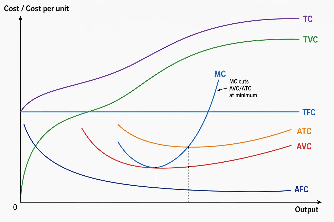
6. Short-Run Cost Curves

Cost is a function of output. In the short run, some inputs are fixed (land, machinery); in the long run, all inputs can be varied (no fixed costs exist).

Mnemonic — “FOSS”: Fixed in Short run, Only variable in long run → no fixed costs in the Long run.

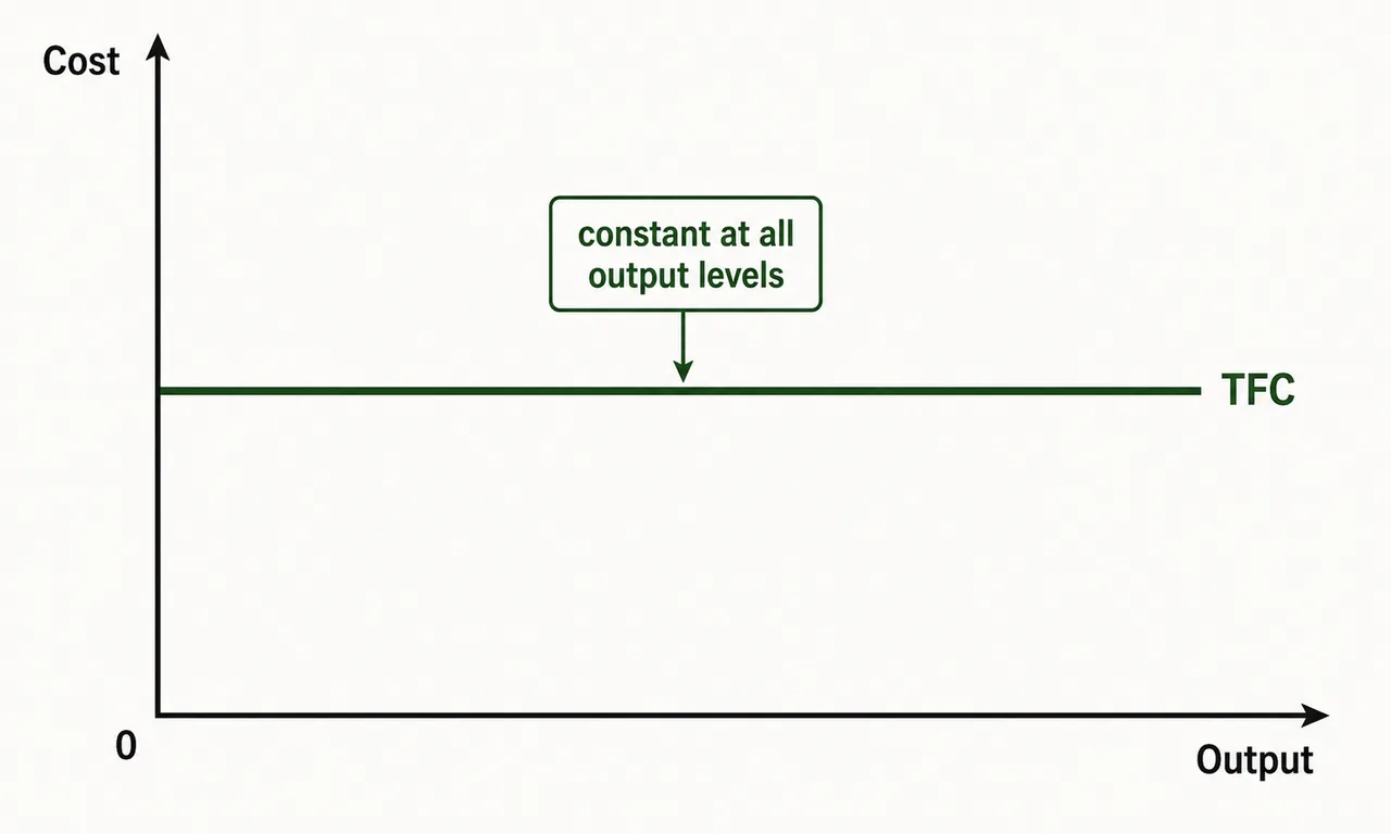
Fixed Cost (FC)

• Does not change with output level
• Incurred even at zero production
• Also called: Overhead Cost, Sunk Cost, Indirect Cost

Cash Fixed Costs	Non-Cash Fixed Costs
Land taxes	Depreciation on machinery
Insurance premiums	Cost of family labour
Interest on loans	Interest on owned fixed capital
Annually hired labour	Management costs

TFC curve: Horizontal straight line parallel to the X-axis.

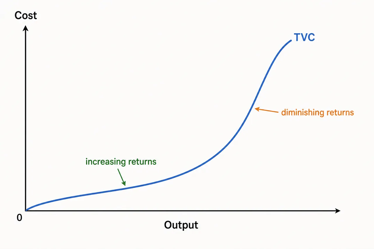
Variable Cost (VC)

• Changes with the level of output
• Falls to zero when production stops
• Also called: Working Cost, Operating Cost, Direct Cost, Prime Cost, Running Cost
• These are second phase costs (incurred during production, unlike establishment costs)

Examples in farming: Seeds, fertilizer, diesel, hired casual labour, feed, irrigation water, pesticides, current repairs.

Farming Expenses = f (farm output)

TVC curve: Inverse S-shape (initially rises slowly due to increasing returns, then rises steeply due to diminishing returns).

Total Cost (TC)

TC = TFC + TVC = Explicit Cost + Implicit Cost

• TC curve has the same shape as TVC, shifted upward by the constant TFC amount.
• At zero output, TC = TFC (fixed costs still apply).

---

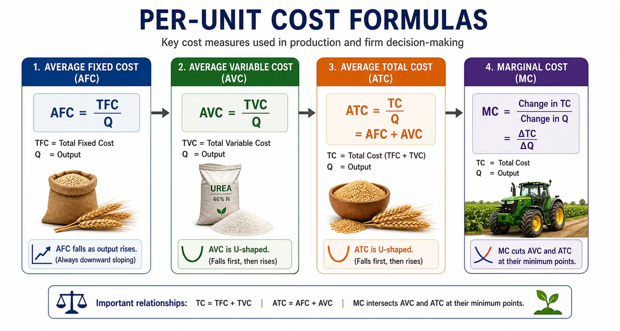
7. Per-Unit Cost Curves

Average Fixed Cost (AFC)

AFC = TFC / Q

• Continuously falls as output increases (same fixed cost spread over more units)
• Shape: Rectangular hyperbola (never touches the X-axis)

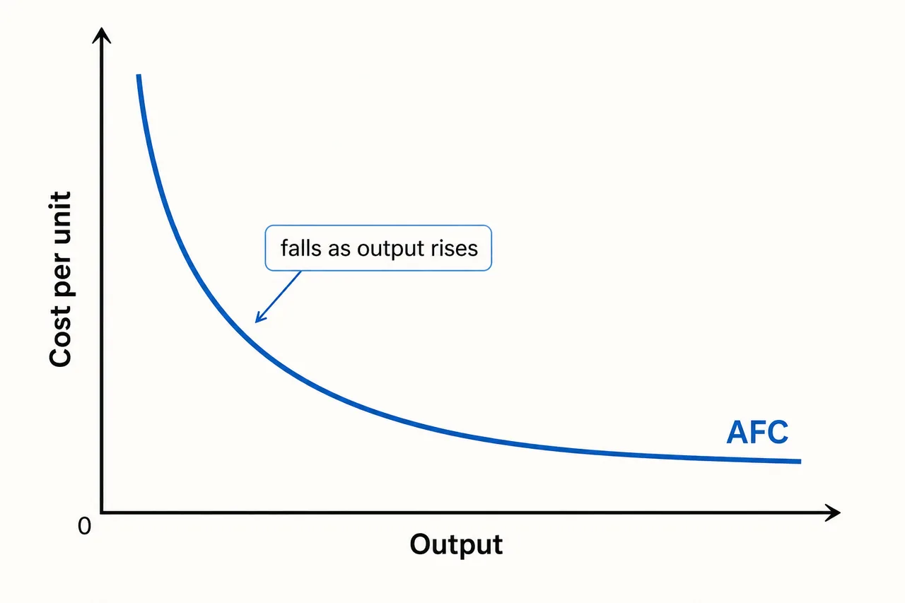
Example: A farmer pays Rs 20,000 in land tax (fixed). If she produces 100 quintals, AFC = Rs 200/quintal. If she produces 400 quintals, AFC = Rs 50/quintal.

Average Variable Cost (AVC)

AVC = TVC / Q

• U-shaped curve (parabolic)
• AVC is the reciprocal of Average Physical Product (APP)
• AVC is minimum when APP is maximum
• Beyond the optimal point, diminishing returns push AVC upward

Example: When a farmer uses the first few bags of urea on wheat, each bag adds a lot of grain (high APP, low AVC). After optimal dosage, extra urea adds less grain (low APP, high AVC).

Average Total Cost (ATC or AC)

ATC = TC / Q = AFC + AVC

• U-shaped curve
• Initially falls because declining AFC dominates
• Later rises because increasing AVC outweighs declining AFC
• The lowest point = most efficient scale of production

Marginal Cost (MC)

MC = Change in TC / Change in Q

• The cost of producing one additional unit
• Marginal Fixed Cost = always zero (FC does not change with output)
• Therefore MC = Marginal Variable Cost only
• MC is independent of the size of fixed cost

Example: A farmer cultivates vegetables on a fixed plot. Adding one more unit of labour costs Rs 500 and produces 2 more quintals. MC = Rs 250/quintal. The rent paid for the land does not affect this calculation.

Key MC relationships:

• MC is U-shaped — falls first (increasing efficiency), then rises (diminishing returns)
• When MPP is maximum, MC is minimum
• When MPP is zero, MC becomes vertical (infinite cost for zero extra output)
• MC intersects AVC and ATC at their minimum points — below the average, it pulls it down; above the average, it pulls it up

---

8. Cost Curve Summary

Mnemonic — “H-I-I-R-U-U-U”: Remember the curve shapes in order: TFC-TVC-TC-AFC-AVC-ATC-MC

Cost Curve	Shape	Key Feature
TFC	Horizontal straight line	Parallel to X-axis, never changes
TVC	Inverse S-shape	Reflects increasing then diminishing returns
TC	Same as TVC (shifted up)	Starts from TFC level, not origin
AFC	Rectangular hyperbola	Always declining, never touches X-axis
AVC	U-shaped	Minimum where APP is maximum
ATC	U-shaped	Minimum point is to the right of AVC minimum
MC	U-shaped	Cuts AVC and ATC at their minimum points

Critical relationships:

• Vertical distance between ATC and AVC = AFC (narrows as output rises)
• When ATC is falling, MC is below ATC
• When ATC is rising, MC is above ATC

Table of Different Costs (Cost in Rupees)

Units of Production	FC	VC	TC = FC + VC	AFC = FC/Q	AVC = VC/Q	ATC = TC/Q	MC = ΔVC/ΔQ
0	25	0	25	∞	-	∞	-
4	25	4	39	6.25	1.00	7.25	1.00
12	25	8	33	2.08	0.66	2.70	0.50
18	25	12	37	1.38	0.66	2.50	0.66
23	25	16	41	1.08	0.69	1.78	0.80
27	25	20	45	0.92	0.74	1.66	1.00
30	25	24	49	0.83	0.80	1.63	1.33
32	25	28	53	0.78	0.87	1.65	2.00
33	25	32	57	0.75	0.96	0.72	4.00

Three key observations from the data:

• Fixed costs remain the same at every production level
• Variable costs change with production level
• Total cost and variable cost increase with rising production

---

9. CACP Cost Concepts in Farm Management

The Commission for Agricultural Costs and Prices (CACP) developed a standardized cost framework used across India. These cost concepts (A1 through C3) form the basis for Minimum Support Price (MSP) determination.

Exam Alert: CACP cost concepts are among the most frequently asked topics in IBPS AFO, FCI, NABARD, and RRB-SO exams.

Cost A1 — The 16 Paid-Out Items

Cost A1 includes all actual cash expenses incurred by the farmer:

1. Value of hired human labour (permanent & casual)
2. Value of owned bullock labour
3. Value of hired bullock labour
4. Value of owned machinery
5. Hired machinery charges
6. Value of fertilizers
7. Value of manure (farm-produced & purchased)
8. Value of seed (farm-produced & purchased)
9. Value of insecticides & fungicides
10. Irrigation charges (owned & hired tube wells, pumping sets)
11. Canal water charges
12. Land revenue, cesses, and other taxes
13. Depreciation on farm implements
14. Depreciation on farm buildings, machinery & irrigation structures
15. Interest on working capital
16. Miscellaneous expenses (artisan wages, ropes, small repairs)

Mnemonic for remembering A1 has 16 items: “A1 = Sweet 16” — the 16 actual paid-out costs.

Building Up from A1 to C3

Cost	Formula	What It Adds
A1	16 paid-out cost items	All actual cash expenses
A2	A1 + Rent for leased land	Lease rental
B1	A1 + Interest on owned fixed capital (excl. land)	Opportunity cost of owned equipment
B2	B1 + Rental value of owned land + Rent for leased land	Opportunity cost of owned land
C1	B1 + Imputed value of family labour	Unpaid family work
C2	B2 + Imputed value of family labour	Most comprehensive cost
C2*	C2 adjusted for statutory/market wage rate	Labour at minimum wage
C3	C2* + 10% of C2*	Managerial input of farmer

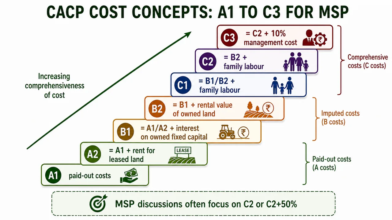
Exam Tip — “ABC progression”:

• A costs = actual paid-out costs
• B costs = A costs + imputed capital costs (no family labour yet)
• C costs = B costs + imputed family labour (the full picture)

Cost C consists of 20 items: Cost A1 (16 items) + Rent for leased land + Imputed value of owned land + Interest on owned fixed capital + Imputed value of family labour

Net Income = Gross Return - Cost C

Cost of Production = Cost C / Output

---

10. Cost of Production vs Cost of Cultivation

Measure	Unit	Primary Use
Cost of Production (CoP)	Rs per quintal	MSP determination
Cost of Cultivation (CoC)	Rs per hectare	Comparing investment intensity across crops/regions

Exam fact (AFO 2017): Cost of Cultivation is measured in Rs per hectare.

Memory trick: Production = per Quintal (product output), Cultivation = per Hectare (land area).

---

Master Summary Table

Concept	Definition (One Line)	Key Fact for Exams
Nominal Cost	Cost at current prices	No inflation adjustment
Real Cost	Cost at constant prices	Removes inflation effect
Opportunity Cost	Value of next best alternative foregone	Introduced by J.S. Mill; zero for free goods
Explicit Cost	Actual cash payments	= Accounting cost
Implicit Cost	Imputed value of own resources	Rent of own land, family labour
Economic Cost	Explicit + Implicit	Always >= Accounting cost
Social Cost	Private cost + externalities	Named by Ronald Coase
Fixed Cost	Does not vary with output	TFC = horizontal line; also called sunk/overhead cost
Variable Cost	Varies with output	TVC = inverse S-shape; also called prime/direct cost
AFC	TFC / Q	Rectangular hyperbola, always declining
AVC	TVC / Q	U-shaped; minimum at maximum APP
ATC	TC / Q = AFC + AVC	U-shaped; minimum to right of AVC minimum
MC	Change in TC / Change in Q	U-shaped; cuts AVC & ATC at their minimums
Cost A1	16 paid-out items	Base for all CACP costs
Cost C2	B2 + family labour	Most comprehensive; basis for MSP
Cost C3	C2* + 10% managerial cost	Highest cost concept
CoP	Cost per quintal	Used for MSP
CoC	Cost per hectare	Used for regional comparison

---

Summary Cheat Sheet

Concept / Topic	Key Details / Explanation
Nominal Cost	Cost at current market prices, no inflation adjustment
Real Cost	Cost at constant (base-year) prices, removes inflation effect
Deflated Cost	Nominal cost divided by price index to remove inflation
Opportunity Cost	Value of the next best alternative foregone; introduced by J.S. Mill; zero for free goods
Explicit Cost	Actual cash payments (hired labour wages, purchased seeds, fertilizer bills); = Accounting cost
Implicit Cost	Imputed value of own resources (rental value of owned land, family labour, interest on own capital)
Economic Cost	Explicit + Implicit cost; always ≥ Accounting cost
Social Cost	Private cost + externalities imposed on society; term coined by Ronald Coase
Separable Cost	Traced to a specific product (e.g., cotton seeds for cotton crop)
Common (Joint) Cost	Shared across multiple products, cannot be separated (e.g., irrigation canal serving multiple crops)
Historical Cost	Original purchase price of a durable asset
Replacement Cost	Difference between current price and original price of the asset
Establishment Cost	One-time costs incurred before production begins (farm buildings, tube wells)
Fixed Cost (FC)	Does not change with output; incurred even at zero production; TFC curve = horizontal line; also called overhead/sunk/indirect cost
Variable Cost (VC)	Changes with output; zero when production stops; TVC curve = inverse S-shape; also called prime/direct/working cost
Total Cost (TC)	TFC + TVC; same shape as TVC shifted up by TFC amount
Average Fixed Cost (AFC)	TFC / Q; continuously falls; shape = rectangular hyperbola (never touches X-axis)
Average Variable Cost (AVC)	TVC / Q; U-shaped; minimum when APP is maximum
Average Total Cost (ATC)	TC / Q = AFC + AVC; U-shaped; minimum point to the right of AVC minimum
Marginal Cost (MC)	ΔTC / ΔQ; U-shaped; intersects AVC and ATC at their minimum points; minimum when MPP is maximum
MC & Fixed Cost	Marginal Fixed Cost = always zero; MC = Marginal Variable Cost only; MC is independent of fixed cost size
Cost Curve Shapes (H-I-I-R-U-U-U)	TFC=Horizontal, TVC=Inverse-S, TC=Inverse-S shifted, AFC=Rectangular hyperbola, AVC=U, ATC=U, MC=U
Cost A1	16 paid-out items (hired labour, seeds, fertilizers, depreciation, irrigation, interest on working capital, etc.) — “A1 = Sweet 16”
Cost A2	A1 + Rent for leased land
Cost B1	A1 + Interest on owned fixed capital (excl. land)
Cost B2	B1 + Rental value of owned land + rent for leased land
Cost C1	B1 + Imputed value of family labour
Cost C2	B2 + Imputed value of family labour — most comprehensive cost; basis for MSP
Cost C3	C2 + 10%* of C2* for managerial input — highest cost concept
Cost of Production (CoP)	Cost per quintal; used for MSP determination
Cost of Cultivation (CoC)	Cost per hectare; used for regional comparison
ABC Progression	A = actual paid-out; B = A + imputed capital costs; C = B + imputed family labour
Net Income Formula	Gross Return − Cost C