🙋🏼Demand and Supply — Core Concepts for Agricultural Economics

Introduction: Why Demand and Supply Matter in Agriculture

Imagine a wheat farmer in Punjab. After a bumper harvest, wheat floods the local mandi. Prices drop. Consumers buy more rotis and less rice. Meanwhile, a drought in Maharashtra reduces onion supply, and onion prices skyrocket across India. These everyday agricultural realities are governed by two fundamental forces: demand and supply.

Understanding these concepts is essential not only for economics exams but also for grasping how agricultural markets, government procurement, MSP decisions, and food security policies actually work.

---

Part 1: Demand

What Is Demand?

Demand is not merely a desire or wish. In economics, demand means the quantity of a good that a buyer is willing and able to purchase at a given price during a specific time period.

Agricultural example: A farmer wants a new tractor (desire). But desire alone is not demand. Only when the farmer has both the willingness and the money (purchasing power) to buy the tractor does it become demand.

Three Essential Characteristics of Demand

Characteristic	Meaning	Agricultural Example
Willingness + Ability to pay	The buyer must want the good AND have the money	A dairy farmer wants cattle feed and can afford it
At a price	Demand is always stated at a specific price	”50 kg of urea at Rs 270/bag” — not just “urea”
Per unit of time	Demand refers to a specific time period	”200 quintals of rice per month” — not just “rice”

Exam Tip: Remember the mnemonic WAP — Willingness, Ability to pay, Price and time period. All three must be present for valid demand.

---

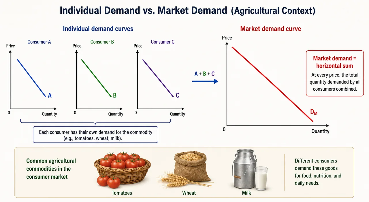
Individual Demand vs Market Demand

Individual demand is the quantity one buyer is willing to purchase at each price level.

Market demand is the horizontal summation of all individual demands at each price level.

Agricultural example: At Rs 40/kg for tomatoes:

• Household A demands 3 kg
• Household B demands 5 kg
• Household C demands 2 kg
• Market demand = 3 + 5 + 2 = 10 kg

At each price, we sum up quantities demanded by every buyer to get market demand.

---

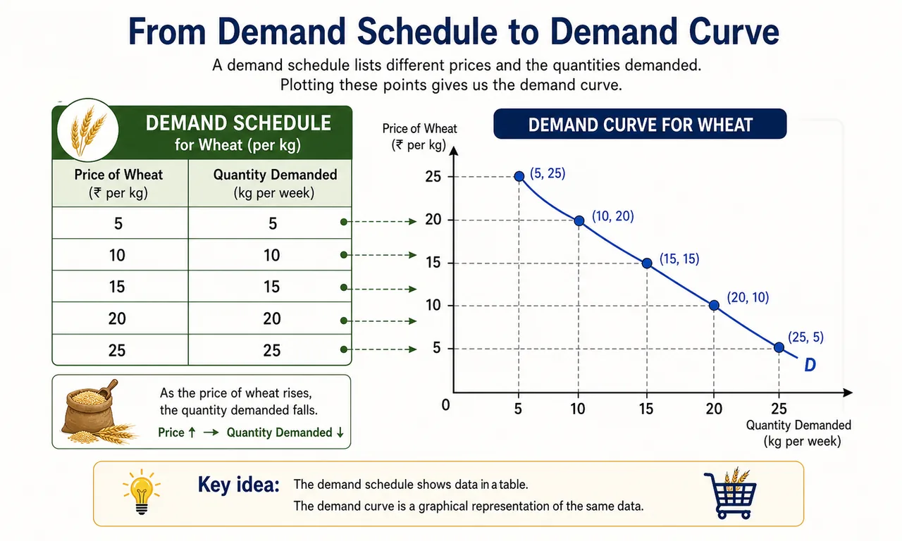
Demand Schedule and Demand Curve

A demand schedule is a table showing quantities demanded at various prices.

Price of Wheat (Rs/kg)	Quantity Demanded (kg/week)
30	100
25	150
20	220
15	300

A demand curve is the graphical representation of a demand schedule. It plots price on the vertical axis and quantity on the horizontal axis. Each point on the curve shows the maximum quantity buyers will purchase at that price.

---

Types of Demand

1. Price Demand

The quantities of a good a consumer is willing to buy at all possible prices, other things remaining constant. This is the most commonly studied form and forms the basis of the demand curve.

Example: How much rice will consumers buy at Rs 40/kg vs Rs 50/kg vs Rs 60/kg?

2. Income Demand

The quantities a consumer is willing to buy at different levels of income, other things remaining constant.

• Normal goods: Demand rises with income (e.g., fruits, dairy products)
• Inferior goods: Demand falls as income rises (e.g., coarse grains like bajra replaced by wheat/rice as income grows)

3. Cross Demand

Demand for a good changes not because of its own price but because of a change in the price of a related good.

Example: When the price of mustard oil rises, consumers switch to sunflower oil. Demand for sunflower oil increases — this is cross demand.

4. Derived Demand

Demand that arises not for the good itself but because it is needed to produce a final product.

Agricultural example: Demand for fertilizers is derived from the demand for food grains. Demand for jute is derived from the demand for jute bags and sacking.

5. Autonomous Demand

Demand that exists independently, for direct consumption, not linked to any other product.

Example: Demand for food grains, vegetables, and milk — these are consumed for their own sake.

Type	Depends On	Agricultural Example
Price demand	Price of the good itself	Rice at different price levels
Income demand	Consumer’s income level	Shift from millets to wheat as income rises
Cross demand	Price of related goods	Mustard oil price rise increases sunflower oil demand
Derived demand	Demand for the final product	Fertilizer demand derived from crop demand
Autonomous demand	Direct consumer need	Demand for vegetables

---

Law of Demand

The law of demand states: as price increases, quantity demanded decreases, and vice versa (other things remaining constant).

In short: price and quantity demanded move in opposite directions.

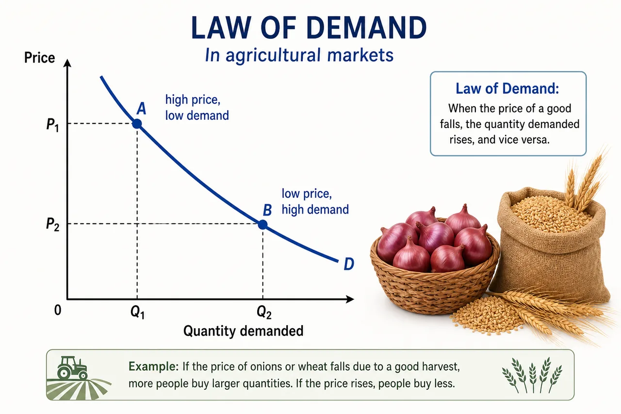
As price falls from PA to PB, quantity demanded increases from QA to QB. The demand curve slopes downward from left to right (negative slope).

Exam Tip: The demand curve slopes downward because of three effects — ISL: Income effect, Substitution effect, Law of diminishing marginal utility.

Why Does the Demand Curve Slope Downward?

1. Income Effect

When the price of wheat falls from Rs 30/kg to Rs 20/kg, a consumer’s purchasing power effectively increases. With the same budget, they can now buy more wheat or spend the savings elsewhere. A price drop makes the consumer “effectively richer.”

2. Substitution Effect

When the price of pulses falls while the price of chicken remains the same, pulses become relatively cheaper. Consumers substitute pulses for chicken, increasing the quantity of pulses demanded. Consumers naturally shift towards the relatively cheaper option.

3. Law of Diminishing Marginal Utility

Each additional unit of a good gives less satisfaction than the previous one. A consumer will buy more units only if the price falls to match the declining marginal utility. This is the fundamental reason behind the law of demand.

---

Changes in Demand: Movement vs Shift

This distinction is critical for exams.

Feature	Movement Along the Curve	Shift of the Curve
Cause	Change in the good’s own price	Change in any factor OTHER than price
Curve position	Stays the same	Moves left or right
Terminology	Extension (price falls) / Contraction (price rises)	Increase (rightward) / Decrease (leftward)
Example	Potato price drops from Rs 30 to Rs 20, quantity demanded rises	Government launches “Eat Millets” campaign, millet demand increases at every price

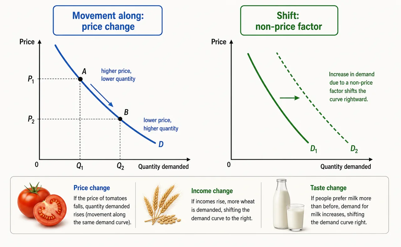
Key Rule: Movement along = price change only. Shift = everything else (income, tastes, related goods’ prices, expectations).

---

Determinants of Demand

Determinant	Effect on Demand	Agricultural Example
Price of the good	Inverse relationship (law of demand)	Higher rice price reduces rice demand
Price of substitutes	Direct relationship	Tur dal price rises, consumers buy more moong dal
Price of complements	Inverse relationship	Tractor price rises, demand for diesel (used with tractors) falls
Income	Direct for normal goods; inverse for inferior goods	Rising rural income increases demand for fruits; decreases demand for coarse grains
Tastes and preferences	Shifts demand curve	Growing health awareness increases demand for organic produce
Future price expectations	Speculative buying or postponement	Farmers hoard onions expecting future price rise

---

Exceptions to the Law of Demand

In these cases, demand does NOT follow the inverse price-quantity relationship:

Exception	Explanation	Example
Giffen Goods	Inferior goods where a strong negative income effect overpowers the substitution effect; demand rises as price rises	Poor families buy more bajra when its price rises because they can no longer afford wheat
Veblen Goods (status symbols)	Higher price increases the good’s prestige value	Expensive Basmati rice varieties seen as status symbols
Speculative buying	Expectation of future price increase causes hoarding	Traders stock up on pulses when prices begin rising, expecting further increases

Exam Tip — Giffen’s Paradox: Named after Sir Robert Giffen, who observed that poor English families bought MORE bread when its price rose (they could no longer afford meat). In Indian agriculture, the same logic applies to coarse cereals for poor households.

---

Part 2: Elasticity of Demand

Elasticity measures how responsive quantity demanded is to a change in a particular factor. It goes beyond direction (up or down) to quantify the magnitude of response.

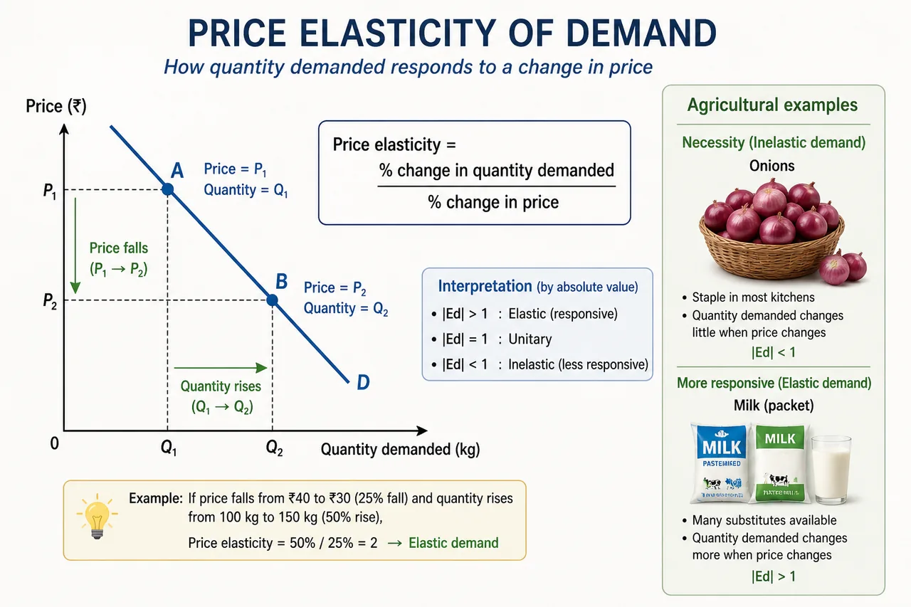
Price Elasticity of Demand

Price elasticity = Percentage change in quantity demanded / Percentage change in price

It answers: “If price changes by 1%, by what percentage does quantity demanded change?”

Income Elasticity of Demand

Income elasticity = Percentage change in quantity demanded / Percentage change in income

• Positive for normal goods (demand rises with income)
• Negative for inferior goods (demand falls as income rises)
• High for luxuries (demand grows faster than income)
• Low for necessities (demand grows slower than income)

Example: As rural income rises, demand for milk (normal good, moderate income elasticity) increases steadily, while demand for coarse millets (inferior good, negative income elasticity) falls.

Cross Elasticity of Demand

Cross elasticity = Percentage change in demand of Good A / Percentage change in price of Good B

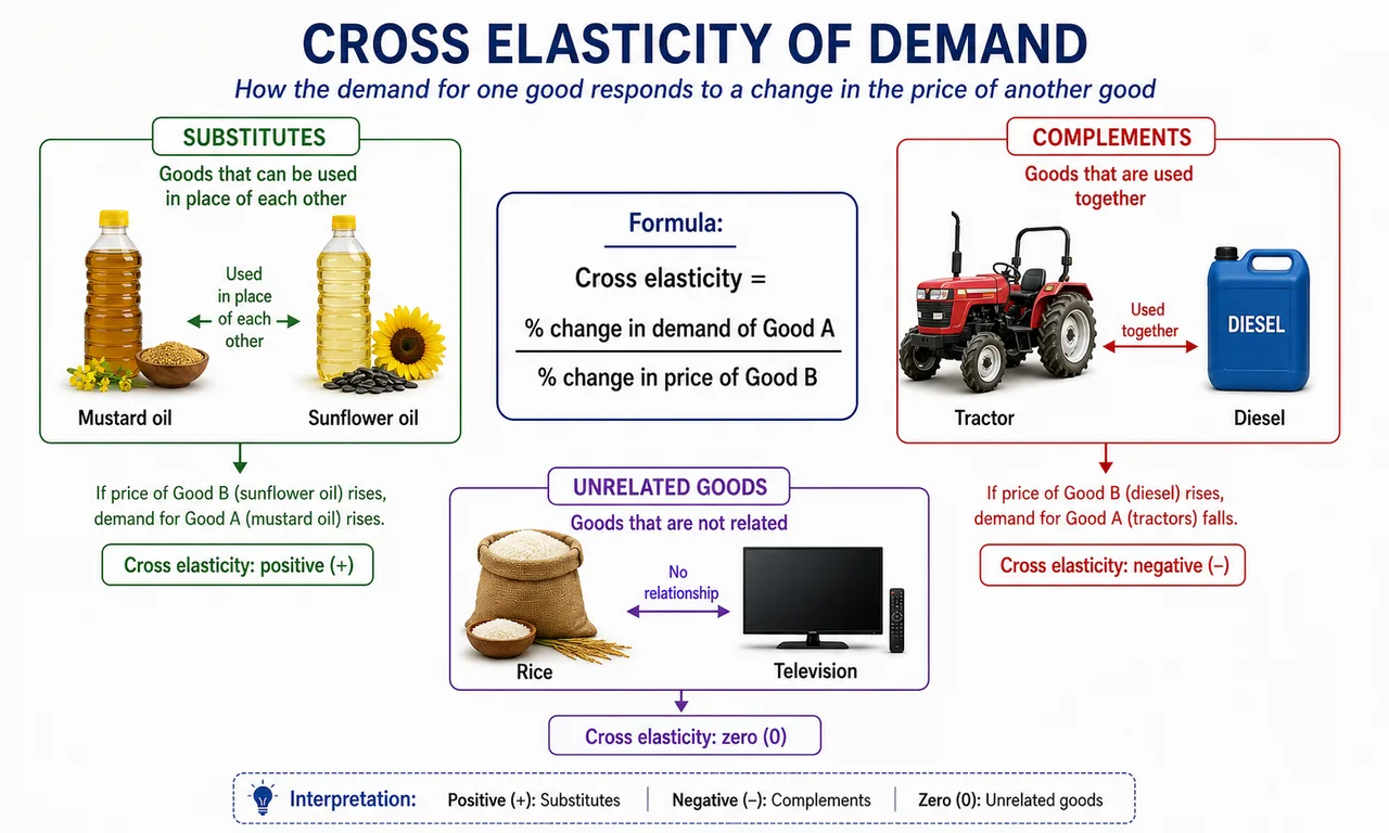
Relationship	Cross Elasticity	Example
Substitutes	Positive (+)	Mustard oil and sunflower oil
Complements	Negative (−)	Tractors and diesel
Unrelated goods	Zero (0)	Rice and televisions

---

Methods of Measuring Elasticity

Method	Description	When to Use
Point elasticity	Measured at a single point on the demand curve	Small/precise price changes
Arc elasticity	Measured between two points on the demand curve (average elasticity over a range)	Large price changes

---

Degrees of Price Elasticity of Demand

Degree	Value	Demand Curve Shape	Example
Perfectly inelastic	E = 0	Vertical line	Essential seeds during sowing season (no substitute)
Perfectly elastic	E = infinity	Horizontal line	Wheat sold in a perfectly competitive mandi (identical quality)
Unitary elastic	E = 1	Rectangular hyperbola	Total expenditure stays constant as price changes
Relatively elastic	E > 1	Flatter curve	Exotic fruits, luxury agricultural products
Relatively inelastic	0 < E < 1	Steeper curve	Food grains, salt, essential vegetables

Exam Mnemonic — PURRE (degrees of elasticity): Perfectly inelastic, Unitary, Relatively elastic, Relatively inelastic, Perfectly Elastic.

---

Factors Determining Price Elasticity of Demand

Factor	Effect	Agricultural Example
Degree of necessity	Necessities have inelastic demand	Wheat, rice, salt — bought regardless of price
Availability of substitutes	More substitutes = more elastic	Groundnut oil (many cooking oil substitutes) is more elastic than salt (no substitute)
Proportion of income spent	Larger share = more elastic	A tractor (large % of income) has more elastic demand than matchboxes
Time period	Long run = more elastic	Farmers can switch crops in the next season if input prices stay high
Number of uses	More uses = more elastic	Sugarcane (sugar, jaggery, ethanol, bagasse) has elastic demand

---

Practical Importance of Elasticity of Demand

Application	How Elasticity Helps	Example
Taxation policy	Taxing inelastic goods generates more revenue with less reduction in sales	Government taxes on tobacco, liquor
Price discrimination by monopolists	Charge higher price where demand is inelastic	APMC mandis charging different fees for essential vs luxury produce
Business pricing	Lower price if demand is elastic; raise price if inelastic	Organic food brands lower prices to expand market share
Trade unions and wages	Workers in inelastic-demand industries have more bargaining power	Dairy workers can push for higher wages since milk demand is inelastic
International trade	Terms of trade depend on elasticity of imports/exports	Marshall-Lerner condition: devaluation improves trade balance only if sum of import and export elasticities exceeds 1
Government agricultural policy	MSP and procurement decisions consider elasticity	Government procures wheat/rice (inelastic demand) to stabilize prices
Advertising decisions	More spending on ads when demand is elastic	Organic food companies invest heavily in marketing
Factor pricing	Factors with inelastic demand command higher prices	Scarce agricultural land near cities earns premium rent

---

Part 3: Supply

What Is Supply?

Supply is the quantity of a good that sellers are willing and able to offer for sale at different prices during a specific time period.

Agricultural example: A rice miller is willing to supply 500 quintals of rice per month at Rs 35/kg but only 300 quintals at Rs 28/kg.

---

Supply vs Stock

Feature	Supply	Stock
Definition	Quantity actually brought to market for sale at a given price	Total quantity available (whether offered for sale or not)
Relationship to market	Active portion offered for sale	Total inventory held by producers
For perishable goods	Supply = Stock (must sell quickly)	Vegetables, fruits, fish — cannot be stored long
For durable goods	Supply may be less than stock	A wheat trader may hold back stock expecting higher prices later

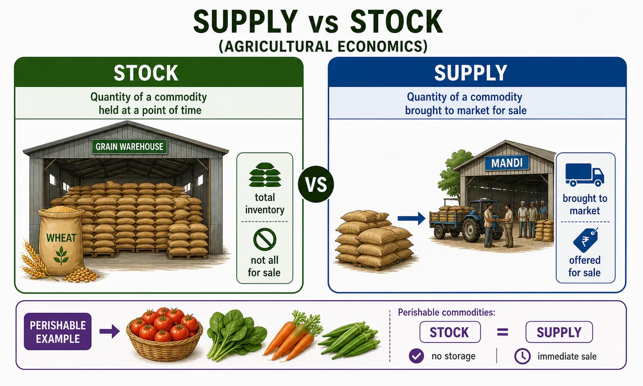
Agricultural insight: During harvest season, farmers often hold back grain stock if current mandi prices are below MSP, waiting for government procurement. Here, stock is large but supply is deliberately restricted.

---

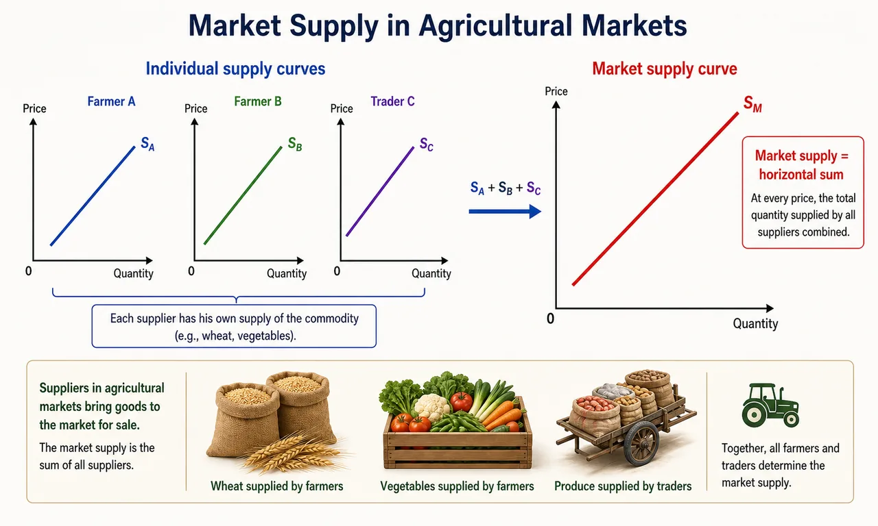
Market Supply

Market supply is the horizontal summation of all individual producers’ supply at each price level — the same concept as market demand but on the supply side.

---

Law of Supply

The law of supply states: as price increases, quantity supplied increases, and vice versa (other things remaining constant).

Supply and price move in the same direction — the opposite of demand. The supply curve slopes upward from left to right.

Why? Higher prices make production more profitable, encouraging producers to supply more.

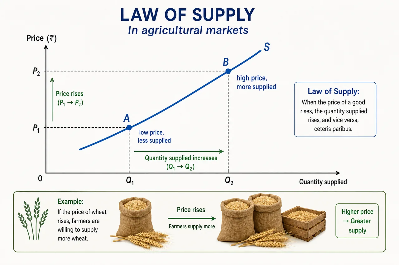
Exam Tip: Demand curve = downward slope (inverse). Supply curve = upward slope (direct). Remember: D for Down, S for Slope-up.

---

Determinants of Supply

Determinant	Effect on Supply	Agricultural Example
Price of the product	Direct — higher price, more supply	Higher MSP for paddy encourages farmers to grow more paddy
Technology	Better tech shifts supply right	Drip irrigation increases crop yield, increasing supply
Input/production costs	Higher costs reduce supply	Rise in fertilizer or diesel prices reduces crop supply
Tax	Increases cost, reduces supply	Higher export tax on onions reduces onion supply to foreign markets
Subsidy	Reduces cost, increases supply	Fertilizer subsidy increases fertilizer supply
Future price expectations	Expected price rise may reduce current supply (hoarding)	Traders hoard pulses expecting price rise after poor monsoon forecast
Price of other goods	Producers shift to more profitable goods	If cotton prices surge, farmers switch from soybean to cotton
Number of producers	More producers = more supply	Entry of new poultry farms increases chicken supply

---

Changes in Supply: Movement vs Shift

Feature	Movement Along Supply Curve	Shift of Supply Curve
Cause	Change in the good’s own price	Change in any factor OTHER than price
Curve position	Stays the same	Moves left or right
Terminology	Extension (price rises) / Contraction (price falls)	Increase (rightward) / Decrease (leftward)
Example	Wheat price rises from Rs 20 to Rs 30, quantity supplied increases	Introduction of HYV seeds increases wheat supply at every price

---

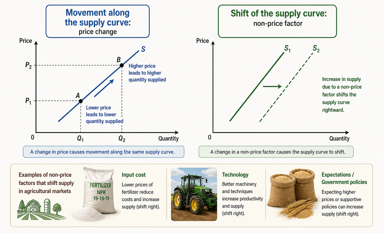
Factors Causing Supply Shifts

Factor	Direction of Shift	Agricultural Example
Fall in input prices	Rightward (increase)	Cheaper fertilizers lower cost, increase crop supply
Technological improvement	Rightward (increase)	Combine harvesters reduce harvesting cost, increase grain supply
Better transport	Rightward (increase)	Cold chain logistics enable supply of perishables to distant markets
Favorable climate	Rightward (increase)	Good monsoon leads to bumper crop, increased supply
Political stability	Rightward (increase)	Stable governance ensures uninterrupted agricultural production
Lower taxes / higher subsidies	Rightward (increase)	Subsidy on drip irrigation increases horticultural supply
Higher taxes / unfavorable policy	Leftward (decrease)	Export ban reduces supply to international markets
Natural disaster	Leftward (decrease)	Floods destroy crops, reducing vegetable supply

---

Determinants of Price Elasticity of Supply

Factor	Effect	Agricultural Example
Time period	Longer time = more elastic	Farmers can switch crops next season; in current season, supply is fixed
Ability to store	Storable goods = more elastic	Wheat (storable) has more elastic supply than tomatoes (perishable)
Factor mobility	Higher mobility = more elastic	If labour can move easily between crops, supply adjusts faster
Marginal cost changes	Rapidly rising costs = less elastic	Expanding irrigation-dependent crops in water-scarce areas faces rising costs
Excess capacity	Spare capacity = more elastic	A flour mill running at 60% capacity can quickly increase output
Infrastructure	Better infrastructure = more elastic	Good roads, cold storage, and irrigation make agricultural supply more responsive
Agriculture vs Industry	Agricultural supply is generally more inelastic	Crops take a full season to grow; factories can adjust output in weeks

Exam Tip: Agricultural supply is inherently more inelastic than industrial supply because crops depend on seasons, weather, and biological growth cycles that cannot be accelerated.

---

Summary Table: Demand vs Supply at a Glance

Concept	Demand	Supply
Definition	Quantity buyers are willing and able to buy	Quantity sellers are willing and able to sell
Law	Price up, quantity down (inverse)	Price up, quantity up (direct)
Curve slope	Downward (left to right)	Upward (left to right)
Movement along curve	Due to change in own price	Due to change in own price
Shift of curve	Due to non-price factors (income, tastes, related prices)	Due to non-price factors (technology, costs, policy)
Elasticity measures	Price, income, cross elasticity	Price elasticity of supply
Agricultural peculiarity	Food demand is generally inelastic	Agricultural supply is generally inelastic (seasonal)

---

Key Formulas for Quick Revision

Formula	Expression
Price Elasticity of Demand	(% change in Qd) / (% change in P)
Income Elasticity of Demand	(% change in Qd) / (% change in Income)
Cross Elasticity of Demand	(% change in Qd of A) / (% change in Price of B)
Marshall-Lerner Condition	Trade balance improves if (Elasticity of exports + Elasticity of imports) > 1

---

Exam-Ready Mnemonics

Mnemonic	Stands For	Concept
WAP	Willingness, Ability to pay, Price and time	Three characteristics of demand
ISL	Income effect, Substitution effect, Law of diminishing marginal utility	Three reasons for downward-sloping demand curve
TIPNS	Tastes, Income, Prices of related goods, Number of buyers, Speculative expectations	Determinants of demand (non-price)
D-Down, S-Slope-up	Demand slopes down, Supply slopes up	Curve directions
PURRE	Perfectly inelastic, Unitary, Relatively elastic, Relatively inelastic, Perfectly Elastic	Five degrees of elasticity

---

Demand and Supply — Video Explanation

---

Summary Cheat Sheet

Concept / Topic	Key Details / Explanation
Definition of Demand	Quantity a buyer is willing and able to purchase at a given price during a specific time period (mnemonic: WAP — Willingness, Ability, Price & time)
Individual vs Market Demand	Market demand = horizontal summation of all individual demands at each price
Demand Schedule & Curve	Schedule is a table; curve plots price (Y-axis) vs quantity (X-axis); slopes downward left to right
Price Demand	Quantities demanded at all possible prices, ceteris paribus — basis of the demand curve
Income Demand	Demand at different income levels; normal goods (direct), inferior goods (inverse)
Cross Demand	Demand changes due to price change of a related good (substitutes or complements)
Derived Demand	Demand arising because the good is needed to produce a final product (e.g., fertiliser demand derived from crop demand)
Autonomous Demand	Demand for direct consumption, independent of other products
Law of Demand	Price up → quantity demanded down (inverse relationship); curve slopes downward due to ISL (Income effect, Substitution effect, LDMU)
Movement vs Shift	Movement along curve = own price change; Shift of curve = non-price factors (income, tastes, related goods, expectations)
Determinants of Demand	Price of good, price of substitutes (direct), price of complements (inverse), income, tastes, future price expectations
Giffen Goods	Inferior goods where income effect > substitution effect; demand rises as price rises (Sir Robert Giffen)
Veblen Goods	Status/prestige goods; higher price increases demand
Price Elasticity of Demand	(% change in Qd) / (% change in P); measures responsiveness of demand to price
Income Elasticity	Positive for normal goods, negative for inferior goods, high for luxuries, low for necessities
Cross Elasticity	Positive for substitutes, negative for complements, zero for unrelated goods
Degrees of Elasticity (PURRE)	Perfectly inelastic (E=0, vertical), Unitary (E=1, rectangular hyperbola), Relatively elastic (E>1), Relatively inelastic (0<E<1), Perfectly elastic (E=∞, horizontal)
Factors Affecting Elasticity	Degree of necessity, availability of substitutes, proportion of income spent, time period, number of uses
Marshall-Lerner Condition	Devaluation improves trade balance only if sum of export and import elasticities > 1
Law of Supply	Price up → quantity supplied up (direct relationship); supply curve slopes upward
Supply vs Stock	Supply = quantity brought to market; Stock = total inventory; for perishable goods, supply = stock
Determinants of Supply	Price, technology, input costs, tax, subsidy, future price expectations, price of other goods, number of producers
Movement vs Shift (Supply)	Movement = own price change (extension/contraction); Shift = non-price factors (technology, costs, policy)
Agricultural Supply	Inherently more inelastic than industrial supply due to seasonal, weather, and biological constraints
Key Formulas	Price Ed = %ΔQd / %ΔP; Income Ed = %ΔQd / %ΔIncome; Cross Ed = %ΔQd(A) / %ΔP(B)