🦹🏼♀️Student's t-Test
One-sample, two-sample, and paired t-tests — formulas, assumptions, worked examples with greengram, potato, and Lucerne data
A breeder develops a new greengram variety expected to yield 13 quintals per hectare. She tests it on only 12 plots — too few for a Z-test. With a small sample and unknown population standard deviation, the t-test is her go-to tool for determining whether the observed yield matches the expected value.
Small Sample Tests
- The entire large sample theory was based on the application of “normal test”. However, if the sample size “n” is small, the distribution of the various statistics, e.g., Z are far from normality and as such “normal test” cannot be applied if “n” is small (
n < 30). - In such cases exact sample tests, we use t-test pioneered by W.S. Gosset (1908) who wrote under the pen name of “Student”, and later on developed and extended by Prof. R.A. Fisher.
The t-test (also called Student’s t-test) is one of the most widely used statistical tests in agricultural research. It is specifically designed for situations where the sample size is small and the population standard deviation is unknown.
t-test for One Samples
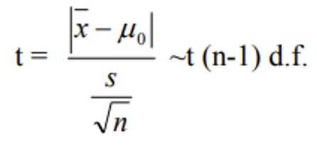
- Let x1, x2, ………. xn be a random sample of size “n” has drawn from a normal population with mean μ and variance σ2 then Student’s t – is defined by the statistic.
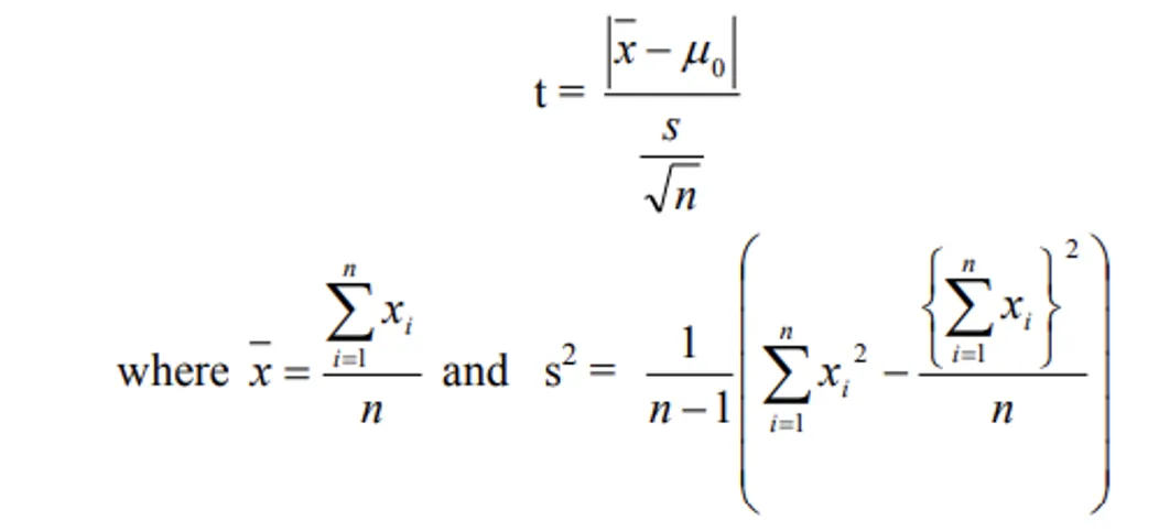
- This test statistic follows a t – distribution with (n-1) degrees of freedom (d.f.). To get the critical value of t we have to refer the table for t-distribution against (n-1) d.f. and the specific level of significance. Comparing the calculated value of t with critical value, we can accept or reject the null hypothesis.
- The Range of t — distribution is -∞ to +∞. Unlike the Z-distribution, the t-distribution has heavier tails, meaning extreme values are more likely. As the sample size increases, the t-distribution approaches the normal distribution.
- ‘T’ test is applicable when number of treatments is 2.
- When sample size is small (n < 30) and S.D. is unknown, use ‘T’ test. This is the key condition that distinguishes the t-test from the Z-test.
- For testing the significance of correlation coefficient, use ‘T’ test.
- When S.D. of population is not known but sample size is more than 30, then use ‘Z’ Test.
TIP
When to use which test?
- Z-test: n > 30 (large sample), σ known or estimated from large sample
- t-test: n < 30 (small sample), σ unknown, also for correlation significance
- F-test: Comparing two or more variances, ANOVA
Example:
- Based on field experiments, a new variety of greengram is expected to give yield of 13 quintals per hectare. The variety was tested on 12 randomly selected farmer fields. The yields (quintal/hectare) were recorded as 14.3, 12.6, 13.7, 10.9,13.7, 12.0, 11.4, 12.0, 13.1, 12.6, 13.4 and 13.1. Do the results conform the expectation?
Solution:
- Null Hypothesis: H0 : μ = μ0 = 13 i.e. the results conform the expectation
- The test statistic becomes
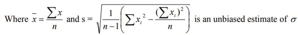
- Let yield = xi (say)
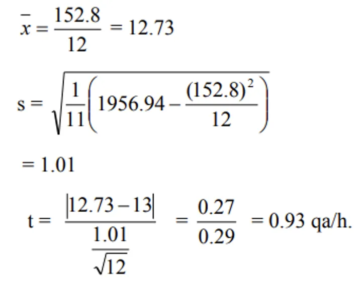
- t-table value at (n-1) = 11 d.f. at 5 percent level of significance is 2.20. Calculated value of t < table value of t, H0 is accepted and we may conclude that the results conform to the expectation.
Since the calculated t-value is less than the critical value, we do not have sufficient evidence to say the yield is different from 13 quintals/hectare. The new variety’s performance is consistent with the expectation.
t-test for Two Samples
The two-sample t-test (also called the independent samples t-test) is used to compare the means of two independent groups when the sample sizes are small and the population standard deviation is unknown.
Assumptions:
- Populations are distributed normally
- Samples are drawn independently and at random
Conditions:
- Standard deviations in the populations are same and not known
- Size of the sample is small
Procedure:
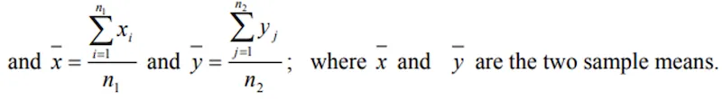
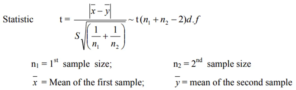
- If two independent samples xi (i = 1, 2, …., n1) and yj (j = 1, 2, ….., n2) of sizes n1 and n2 have been drawn from two normal populations with means μ1 and μ2 respectively.
- Null hypothesis H0: μ1 = μ2
- The null hypothesis states that the population means of the two groups are identical, so their difference is zero.
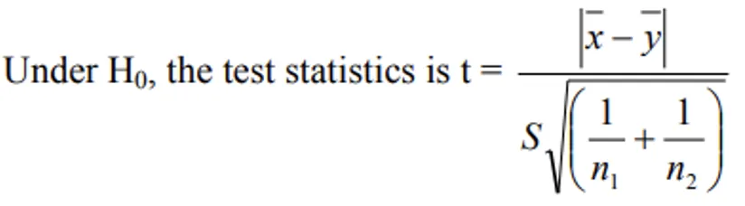
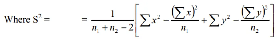
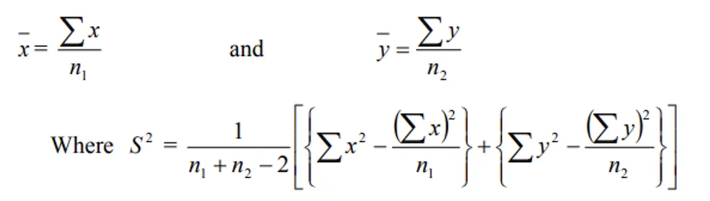
- where s12 and s22 are the variances of the first and second samples respectively.
- Which follows Student’s t – distribution with (n1 + n2 - 2) d.f. If calculated value of |t| < table value of t with (n1 + n2 - 2) d.f. at specified level of significance, then the null hypothesis is accepted otherwise rejected.
Note that the degrees of freedom for the two-sample t-test is (n1 + n2 - 2), which accounts for the two constraints (the two sample means).
Example:
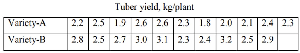
- Two verities of potato plants (A and B) yielded tubers are shown in the following table. Does the mean weight of tubers of the variety “A” significantly differ from that of variety “B”?
Solution:
- Hypothesis H0 : μ1 = μ2 i.e. the mean weight of tubers of the variety “A” do not significantly differ from the variety “B”.
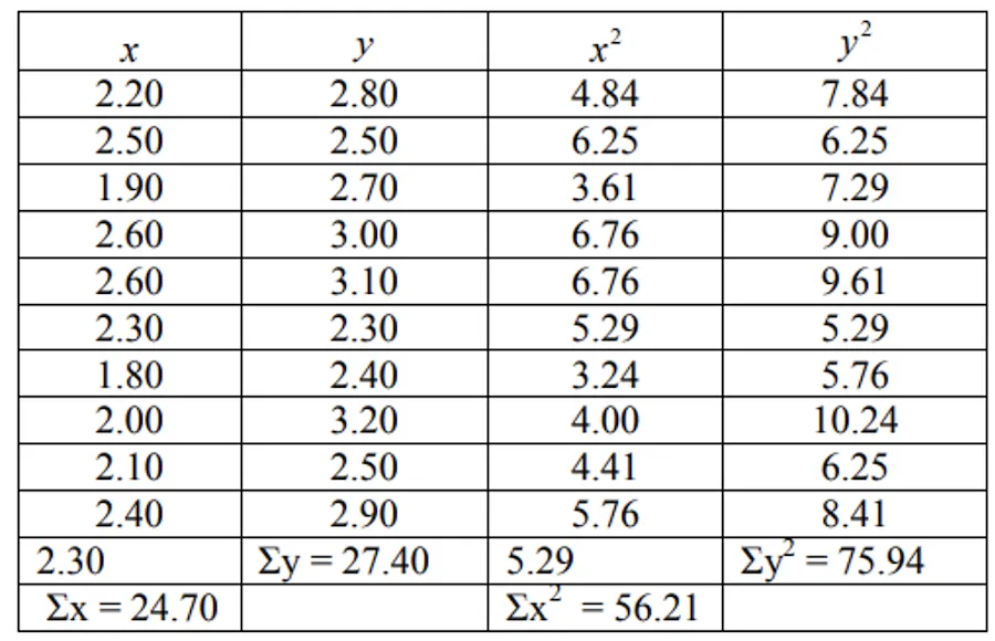
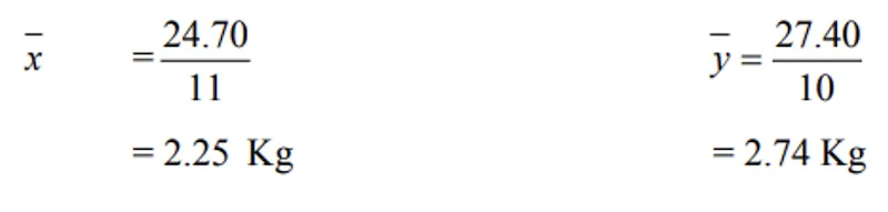
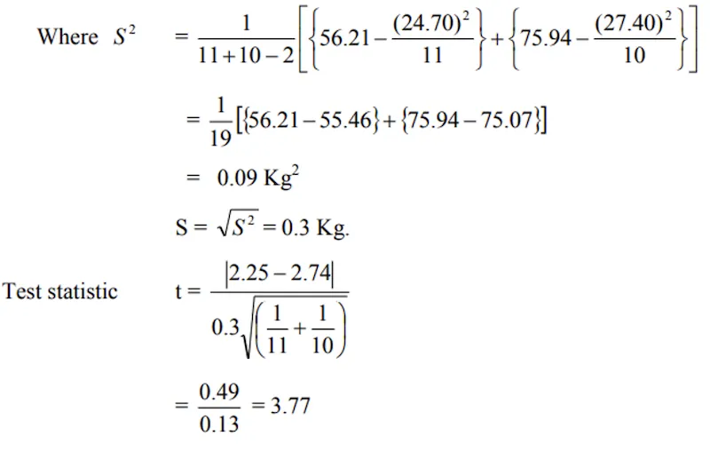
- Calculated value of t = 3.77. Table value of t for 19 d.f. at 5 % level of significance is 2.09 Since the calculated value of t > table value of t, the null hypothesis is rejected and hence we conclude that the mean number of tubes of the variety “A” significantly differ from the variety “B”.
Paired t – test
The paired t-test is used when the two samples are not independent but are related — typically measurements taken on the same subject before and after a treatment or under two different conditions.
- The paired t-test is generally used when measurements are taken from the same subject before and after some manipulation such as injection of a drug.
- For example, you can use a paired t test to determine the significance of a difference in blood pressure before and after administration of an experimental pressure substance.
Assumptions
- Populations are distributed normally
- Samples are drawn independently and at random
Conditions
- Samples are related with each other
- Sizes of the samples are small and equal
- Standard deviations in the populations are equal and not known
Hypothesis
- H0: μd = 0
This null hypothesis states that the mean difference between paired observations is zero, i.e., there is no effect of the treatment.
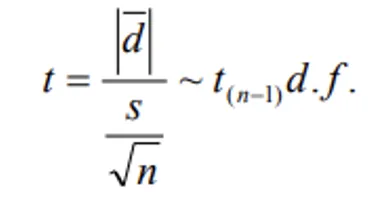
- Under H0, the test statistic becomes,
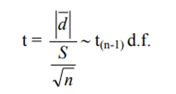
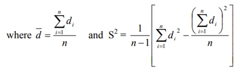
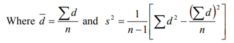
- Where
- S2 is variance of the deviations
- n = sample size; where di = xi - yi (i = 1,2, ……, n)
- If calculated value of |t| < table value of t for (n-1) d.f. at α % level of significance, then the null hypothesis is accepted and hence we conclude that the two samples may belong to the same population. Otherwise, the null hypothesis rejected.
Example
- The average number of seeds set per pod in Lucerne were determined for top flowers and bottom flowers in ten plants.
- The values observed were as follows:
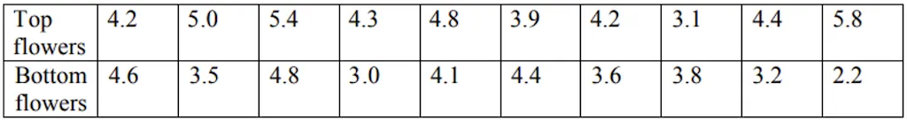
- Test whether there is any significant difference between the top and bottom flowers with respect to average numbers of seeds set per pod.
Solution:
- Null Hypothesis H0: μd = 0
- Under H0 becomes, the test statistic is
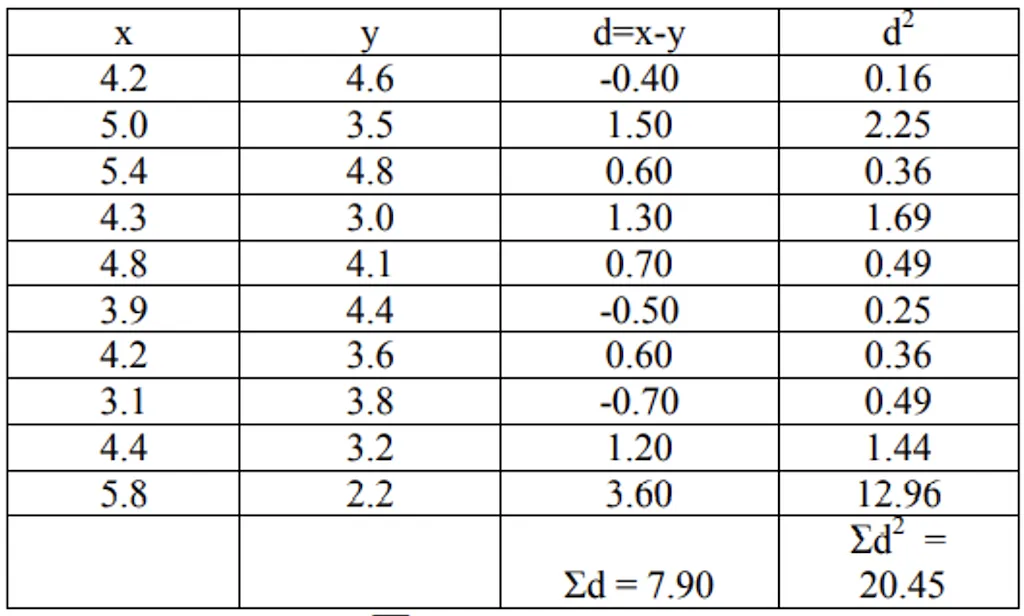
- Calculated value of t = 1.65
- Table value of t for 9 d.f. at 5% level of significance is 2.26
- Calculated value of t < table value of t, the null hypothesis is accepted and we conclude that there is no significant difference between the top and bottom flowers with respect to average numbers of seeds set per pod.
Since the calculated t (1.65) is well below the critical value (2.26), the observed difference is likely due to random variation rather than a genuine difference in seed setting between top and bottom flowers.
Summary Table
| Test Type | When to Use | d.f. | Hypothesis |
|---|---|---|---|
| One-sample t-test | Compare sample mean with known value | n - 1 | H0: μ = μ0 |
| Two-sample t-test | Compare means of two independent groups | n1 + n2 - 2 | H0: μ1 = μ2 |
| Paired t-test | Compare paired/related measurements | n - 1 | H0: μd = 0 |
| Concept | Key Point | Exam Tip |
|---|---|---|
| Discoverer | W.S. Gosset (“Student”), extended by R.A. Fisher | Pen name = Student |
| When to use | n < 30, σ unknown | Small sample, unknown S.D. |
| Range | -∞ to +∞ | Heavier tails than Z |
| Number of treatments | 2 maximum | Use F-test/ANOVA for more |
| vs Z-test | n < 30 → t-test; n > 30 and σ known → Z-test | Key decision criterion |
| For correlation | Use t-test to test significance of r | d.f. = n - 2 |
TIP
Quick decision guide: Sample small (n < 30) and σ unknown? Use t-test. Sample large (n > 30)? Use Z-test. More than 2 groups? Use F-test (ANOVA).
Summary Cheat Sheet
| Concept / Topic | Key Details |
|---|---|
| Student’s t-test | Pioneered by W.S. Gosset (1908, pen name “Student”) |
| Extended by | Prof. R.A. Fisher |
| When to use | n < 30 (small sample), σ unknown |
| Range of t | -∞ to +∞ (heavier tails than Z-distribution) |
| Max treatments | 2 — use F-test/ANOVA for more |
| One-sample t-test | Compare sample mean with known value; d.f. = n - 1 |
| Two-sample t-test | Compare means of two independent groups; d.f. = n₁ + n₂ - 2 |
| Paired t-test | Compare related/paired measurements; d.f. = n - 1 |
| Paired t-test H₀ | μ_d = 0 (mean difference = zero) |
| Two-sample assumptions | Normal populations, independent random samples, equal unknown σ |
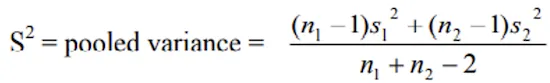
| Pooled variance | s² = (SS₁ + SS₂) / (n₁ + n₂ - 2) |
| For correlation | t-test tests significance of r; d.f. = n - 2 |
| vs Z-test | n < 30 → t-test; n > 30 and σ known → Z-test |
| Decision rule | |
| t approaches Z | As sample size increases, t-distribution → normal |
| Practical use | Greengram yield testing, potato variety comparison, Lucerne seed set |
| Key distinction | t-test for small samples with unknown S.D. |
Pro Content Locked
Upgrade to Pro to access this lesson and all other premium content.
₹2388 billed yearly
- All Agriculture & Banking Courses
- AI Lesson Questions (100/day)
- AI Doubt Solver (50/day)
- Glows & Grows Feedback (30/day)
- AI Section Quiz (20/day)
- 22-Language Translation (30/day)
- Recall Questions (20/day)
- AI Quiz (15/day)
- AI Quiz Paper Analysis
- AI Step-by-Step Explanations
- Spaced Repetition Recall (FSRS)
- AI Tutor
- Immersive Text Questions
- Audio Lessons — Hindi & English
- Mock Tests & Previous Year Papers
- Summary & Mind Maps
- XP, Levels, Leaderboard & Badges
- Generate New Classrooms
- Voice AI Teacher (AgriDots Live)
- AI Revision Assistant
- Knowledge Gap Analysis
- Interactive Revision (LangGraph)
🔒 Secure via Razorpay · Cancel anytime · No hidden fees
A breeder develops a new greengram variety expected to yield 13 quintals per hectare. She tests it on only 12 plots — too few for a Z-test. With a small sample and unknown population standard deviation, the t-test is her go-to tool for determining whether the observed yield matches the expected value.
Small Sample Tests
- The entire large sample theory was based on the application of “normal test”. However, if the sample size “n” is small, the distribution of the various statistics, e.g., Z are far from normality and as such “normal test” cannot be applied if “n” is small (
n < 30). - In such cases exact sample tests, we use t-test pioneered by W.S. Gosset (1908) who wrote under the pen name of “Student”, and later on developed and extended by Prof. R.A. Fisher.
The t-test (also called Student’s t-test) is one of the most widely used statistical tests in agricultural research. It is specifically designed for situations where the sample size is small and the population standard deviation is unknown.
t-test for One Samples
- Let x1, x2, ………. xn be a random sample of size “n” has drawn from a normal population with mean μ and variance σ2 then Student’s t – is defined by the statistic.
- This test statistic follows a t – distribution with (n-1) degrees of freedom (d.f.). To get the critical value of t we have to refer the table for t-distribution against (n-1) d.f. and the specific level of significance. Comparing the calculated value of t with critical value, we can accept or reject the null hypothesis.
- The Range of t — distribution is -∞ to +∞. Unlike the Z-distribution, the t-distribution has heavier tails, meaning extreme values are more likely. As the sample size increases, the t-distribution approaches the normal distribution.
- ‘T’ test is applicable when number of treatments is 2.
- When sample size is small (n < 30) and S.D. is unknown, use ‘T’ test. This is the key condition that distinguishes the t-test from the Z-test.
- For testing the significance of correlation coefficient, use ‘T’ test.
- When S.D. of population is not known but sample size is more than 30, then use ‘Z’ Test.
TIP
When to use which test?
- Z-test: n > 30 (large sample), σ known or estimated from large sample
- t-test: n < 30 (small sample), σ unknown, also for correlation significance
- F-test: Comparing two or more variances, ANOVA
Example:
- Based on field experiments, a new variety of greengram is expected to give yield of 13 quintals per hectare. The variety was tested on 12 randomly selected farmer fields. The yields (quintal/hectare) were recorded as 14.3, 12.6, 13.7, 10.9,13.7, 12.0, 11.4, 12.0, 13.1, 12.6, 13.4 and 13.1. Do the results conform the expectation?
Solution:
- Null Hypothesis: H0 : μ = μ0 = 13 i.e. the results conform the expectation
- The test statistic becomes
- Let yield = xi (say)
- t-table value at (n-1) = 11 d.f. at 5 percent level of significance is 2.20. Calculated value of t < table value of t, H0 is accepted and we may conclude that the results conform to the expectation.
Since the calculated t-value is less than the critical value, we do not have sufficient evidence to say the yield is different from 13 quintals/hectare. The new variety’s performance is consistent with the expectation.
t-test for Two Samples
The two-sample t-test (also called the independent samples t-test) is used to compare the means of two independent groups when the sample sizes are small and the population standard deviation is unknown.
Assumptions:
- Populations are distributed normally
- Samples are drawn independently and at random
Conditions:
- Standard deviations in the populations are same and not known
- Size of the sample is small
Procedure:
- If two independent samples xi (i = 1, 2, …., n1) and yj (j = 1, 2, ….., n2) of sizes n1 and n2 have been drawn from two normal populations with means μ1 and μ2 respectively.
- Null hypothesis H0: μ1 = μ2
- The null hypothesis states that the population means of the two groups are identical, so their difference is zero.
- where s12 and s22 are the variances of the first and second samples respectively.
- Which follows Student’s t – distribution with (n1 + n2 - 2) d.f. If calculated value of |t| < table value of t with (n1 + n2 - 2) d.f. at specified level of significance, then the null hypothesis is accepted otherwise rejected.
Note that the degrees of freedom for the two-sample t-test is (n1 + n2 - 2), which accounts for the two constraints (the two sample means).
Example:
- Two verities of potato plants (A and B) yielded tubers are shown in the following table. Does the mean weight of tubers of the variety “A” significantly differ from that of variety “B”?
Solution:
- Hypothesis H0 : μ1 = μ2 i.e. the mean weight of tubers of the variety “A” do not significantly differ from the variety “B”.
- Calculated value of t = 3.77. Table value of t for 19 d.f. at 5 % level of significance is 2.09 Since the calculated value of t > table value of t, the null hypothesis is rejected and hence we conclude that the mean number of tubes of the variety “A” significantly differ from the variety “B”.
Paired t – test
The paired t-test is used when the two samples are not independent but are related — typically measurements taken on the same subject before and after a treatment or under two different conditions.
- The paired t-test is generally used when measurements are taken from the same subject before and after some manipulation such as injection of a drug.
- For example, you can use a paired t test to determine the significance of a difference in blood pressure before and after administration of an experimental pressure substance.
Assumptions
- Populations are distributed normally
- Samples are drawn independently and at random
Conditions
- Samples are related with each other
- Sizes of the samples are small and equal
- Standard deviations in the populations are equal and not known
Hypothesis
- H0: μd = 0
This null hypothesis states that the mean difference between paired observations is zero, i.e., there is no effect of the treatment.
- Under H0, the test statistic becomes,
- Where
- S2 is variance of the deviations
- n = sample size; where di = xi - yi (i = 1,2, ……, n)
- If calculated value of |t| < table value of t for (n-1) d.f. at α % level of significance, then the null hypothesis is accepted and hence we conclude that the two samples may belong to the same population. Otherwise, the null hypothesis rejected.
Example
- The average number of seeds set per pod in Lucerne were determined for top flowers and bottom flowers in ten plants.
- The values observed were as follows:
- Test whether there is any significant difference between the top and bottom flowers with respect to average numbers of seeds set per pod.
Solution:
- Null Hypothesis H0: μd = 0
- Under H0 becomes, the test statistic is
- Calculated value of t = 1.65
- Table value of t for 9 d.f. at 5% level of significance is 2.26
- Calculated value of t < table value of t, the null hypothesis is accepted and we conclude that there is no significant difference between the top and bottom flowers with respect to average numbers of seeds set per pod.
Since the calculated t (1.65) is well below the critical value (2.26), the observed difference is likely due to random variation rather than a genuine difference in seed setting between top and bottom flowers.
Summary Table
| Test Type | When to Use | d.f. | Hypothesis |
|---|---|---|---|
| One-sample t-test | Compare sample mean with known value | n - 1 | H0: μ = μ0 |
| Two-sample t-test | Compare means of two independent groups | n1 + n2 - 2 | H0: μ1 = μ2 |
| Paired t-test | Compare paired/related measurements | n - 1 | H0: μd = 0 |
| Concept | Key Point | Exam Tip |
|---|---|---|
| Discoverer | W.S. Gosset (“Student”), extended by R.A. Fisher | Pen name = Student |
| When to use | n < 30, σ unknown | Small sample, unknown S.D. |
| Range | -∞ to +∞ | Heavier tails than Z |
| Number of treatments | 2 maximum | Use F-test/ANOVA for more |
| vs Z-test | n < 30 → t-test; n > 30 and σ known → Z-test | Key decision criterion |
| For correlation | Use t-test to test significance of r | d.f. = n - 2 |
TIP
Quick decision guide: Sample small (n < 30) and σ unknown? Use t-test. Sample large (n > 30)? Use Z-test. More than 2 groups? Use F-test (ANOVA).
Summary Cheat Sheet
| Concept / Topic | Key Details |
|---|---|
| Student’s t-test | Pioneered by W.S. Gosset (1908, pen name “Student”) |
| Extended by | Prof. R.A. Fisher |
| When to use | n < 30 (small sample), σ unknown |
| Range of t | -∞ to +∞ (heavier tails than Z-distribution) |
| Max treatments | 2 — use F-test/ANOVA for more |
| One-sample t-test | Compare sample mean with known value; d.f. = n - 1 |
| Two-sample t-test | Compare means of two independent groups; d.f. = n₁ + n₂ - 2 |
| Paired t-test | Compare related/paired measurements; d.f. = n - 1 |
| Paired t-test H₀ | μ_d = 0 (mean difference = zero) |
| Two-sample assumptions | Normal populations, independent random samples, equal unknown σ |
| Pooled variance | s² = (SS₁ + SS₂) / (n₁ + n₂ - 2) |
| For correlation | t-test tests significance of r; d.f. = n - 2 |
| vs Z-test | n < 30 → t-test; n > 30 and σ known → Z-test |
| Decision rule | |
| t approaches Z | As sample size increases, t-distribution → normal |
| Practical use | Greengram yield testing, potato variety comparison, Lucerne seed set |
| Key distinction | t-test for small samples with unknown S.D. |
Knowledge Check
Take a dynamically generated quiz based on the material you just read to test your understanding and get personalized feedback.
Lesson Doubts
Ask questions, get expert answers