🥷Chi-Square Test (Non-Parametric Test)
Goodness of fit, independence of attributes, contingency tables, Yates correction — with Mendelian genetics and Datura examples
A plant geneticist crosses two pea varieties and observes 315 round-yellow, 108 round-green, 101 wrinkled-yellow, and 32 wrinkled-green seeds. Do these counts fit the expected 9:3:3:1 Mendelian ratio? The Chi-square test is the tool that answers this question — it compares observed frequencies with expected ones to determine if the difference is due to chance or a real departure from theory.
- The various tests of significance studied earlier such that as Z-test, t-test, F-test were based on the assumption that the samples were drawn from normal population. Under this assumption the various statistics were normally distributed. These tests work well when we know (or can reasonably assume) the shape of the population distribution.
- Since the procedure of testing the significance requires the knowledge about the type of population or parameters of population from which random samples have been drawn, these tests are known as
parametric tests. Parametric tests rely on specific distributional assumptions and estimate population parameters like the mean and variance.
- But there are many practical situations in which the assumption of any kind about the distribution of population or its parameter is not possible to make. The alternative technique where no assumption about the distribution or about parameters of population is made are known as non-parametric tests. These are also called distribution-free tests because they do not require the data to follow any specific probability distribution.
- Chi-square test is an example of the non-parametric test.
- Chi-square distribution is a distribution free test.
- Chi-square distribution was first discovered by Helmert in 1876 and later independently by Karl Pearson in 1900. Karl Pearson developed it as a practical tool for testing how well observed data fits a theoretical expectation, which is why it is sometimes called Pearson’s chi-square test.
- The range of chi-square distribution is 0 to ∞. Since chi-square is calculated as a sum of squared terms, it can never be negative. A value of zero means perfect agreement between observed and expected frequencies, while larger values indicate greater discrepancy.
- If observed frequency is equal to expected one than the value of χ2 static is zero.
- Measurement data: the data obtained by actual measurement is called measurement data. For example, height, weight, age, income, area etc. This type of data is typically continuous in nature and can take any value within a range.
- Enumeration data: the data obtained by enumeration or counting is called enumeration data. For example, number of blue flowers, number of intelligent boys, number of curled leaves, etc. This type of data involves counting items that fall into specific categories.
- χ2 – test is
used for enumeration datawhich generally relate to discrete variable whereas t-test and standard normal deviate tests are used for measuremental data which generally relate to continuous variable. This is an important distinction — chi-square is designed to work with categorical or count data, not with measurements on a continuous scale. - χ2 – test can be used to know whether the given objects are segregating in a theoretical ratio or whether the two attributes are independent in a contingency table. In agricultural genetics, for example, chi-square is commonly used to verify whether the offspring of a cross follow the expected Mendelian ratios (such as 3:1 or 9:3:3:1).
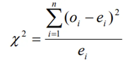
- The expression for χ2–test for goodness of fit:
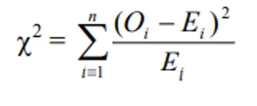
- Where
- Oi = observed frequencies
- Ei = expected frequencies
- n = number of cells (or classes)
- Which follows a chi-square distribution with (n-1) degrees of freedom.
- The null hypothesis H0 = the observed frequencies are in agreement with the expected frequencies. In other words, we start by assuming that there is no significant difference between what we observed and what we expected based on theory.
- If the calculated value of χ2 < Table value of χ2 with (n-1) d.f. at specified level of significance (α), we accept H0 otherwise we do not accept H0. When the calculated value exceeds the table value, it means the difference between observed and expected frequencies is too large to be explained by chance alone, and we reject the null hypothesis.
Conditions for the validity of χ2 – test
- The validity of χ2-test of goodness of fit between theoretical and observed, the following conditions must be satisfied. These conditions are essential for the chi-square approximation to be reliable:
- The sample observations should be independent — the inclusion of one observation should not affect another.
- Constraints on the cell frequencies, if any, should be linear ∑Oi = ∑Ei
- N, the total frequency should be reasonably large, say greater than 50. With small sample sizes, the chi-square approximation becomes unreliable.
- If any theoretical (expected) cell frequency is less than 5, then for the application of chi-square test it is pooled with the preceding or succeeding frequency so that the pooled frequency is more than 5 and finally adjust for the d.f. lost in pooling. This pooling (also called combining classes) is necessary because very small expected frequencies distort the chi-square statistic and lead to inaccurate results.
WARNING
Two critical conditions for valid chi-square test: total frequency N > 50 and all expected cell frequencies ≥ 5. If expected frequency < 5, pool adjacent classes before applying the test.
Applications of Chi-square Test
- Testing the
independence of attributes— to determine whether two categorical variables are related or independent of each other. - To test the
goodness of fit(it tells you if your sample data represents the data you would expect to find in the actual population). This is widely used in genetics to verify Mendelian ratios. - Testing of linkage in genetic problems — to check whether two genes are inherited independently or are linked on the same chromosome.
- Comparison of sample variance with population variance
- Testing the
homogeneity of variancesUPPSC 2021 - Testing the
homogeneity of correlation coefficient - The test whether theory fits well in practical can be judged by Chi square test
Test for independence of two Attributes of (2x2) Contingency Table
- A characteristic which cannot be measured but can only be classified to one of the different levels of the character under consideration is called an attribute. For example, eye colour, intelligence level, or flower colour are attributes — they are qualitative, not quantitative.
- 2x2 contingency table: When the individuals (objects) are classified into two categories with respect to each of the two attributes then the table showing frequencies distributed over 2x2 classes is called 2x2 contingency table. This is the simplest form of a contingency table and is extremely common in agricultural and biological research.
- Suppose the individuals are classified according to two attributes say intelligence (A) and colour (B). The distribution of frequencies over cells is shown in the following table.
| A \ B | A1 | A2 | Row totals |
|---|---|---|---|
| B1 | a | b | R1 = (a+b) |
| B2 | c | d | R2 = (c+d) |
| Column total | C1 = (a+c) | C2 = (b+d) | N = (R1+R2) or (C1+C2) |
- Where
- R1 and R2 are the marginal totals of 1st row and 2nd row
- C1 and C2 are the marginal totals of 1st column and 2nd column
- N = grand total
- The null hypothesis H0: the two attributes are independent (if the colour is not dependent on intelligent). In other words, we assume that knowing one attribute tells us nothing about the other attribute.
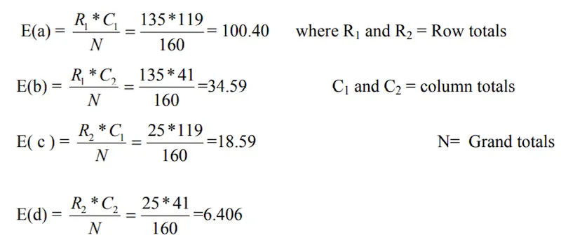
- Based on above H0, the expected frequencies are calculated as follows.
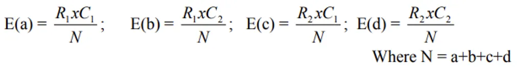
The expected frequency for any cell is calculated by multiplying the corresponding row total by the column total and dividing by the grand total. This formula is based on the probability rule for independent events.
- The degrees of freedom for m x n contingency table is (m - 1) x (n - 1)
- The degrees of freedom for 2 x 2 contingency table is (2 - 1)(2 - 1) = 1
- This method is applied for all r x c contingency tables to get the expected frequencies.
- The degrees of freedom for r x c contingency table is (r - 1) x (c - 1)
- If the calculated value of χ2 < table value of χ2 at certain level of significance, then H0 is accepted otherwise we do not accept H0.
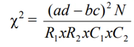
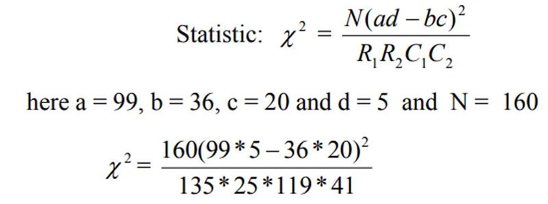
- The alternative formula for calculating χ2 in 2 x 2 contingency table is:
Example
- Examine the following table showing the number of plants having certain characters, test the hypothesis that the flower colour is independent of the shape of leaf.
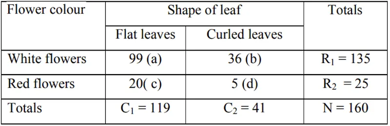
Solution:
- Null hypothesis H0: attributes “flower colour” and “shape of leaf” are independent of each other.
- Under H0 the statistic is
- Expected frequencies are calculated as follows.
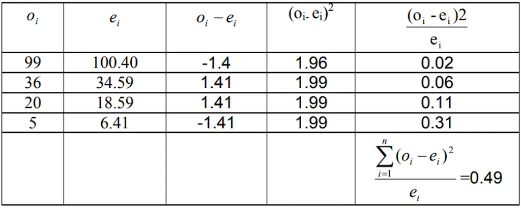
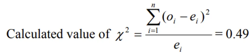
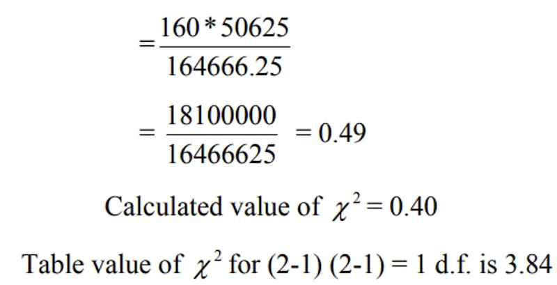
Direct Method:
- Calculated value of χ2 < Table value of χ2 at 5% LOS for 1 d.f., Null hypothesis is accepted and hence we conclude that two characters, flower colour and shape of leaf are independent of each other.
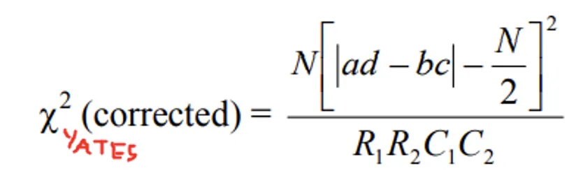
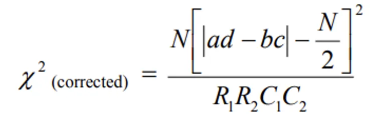
- Yates correction for continuity in a 2 x 2 contingency table
- In a 2 x 2 contingency table, the number of d.f. is (2 - 1) x (2 - 1) = 1. If any one of Expected cell frequency is less than 5, then we use of pooling method for χ2–test results with ‘0’ d.f. (since 1 d.f. is lost in pooling) which is meaningless. In this case we apply a correction due to Yates, which is usually known a
Yates Correction for Continuity. This correction compensates for the fact that a discrete distribution (frequencies) is being approximated by a continuous distribution (chi-square). It makes the test slightly more conservative (less likely to falsely reject H0).
- Yates correction consists of the following steps:
- Add 0.5 to the cell frequency which is the least.
- Adjust the remaining cell frequencies in such a way that the row and column totals are not changed. It can be shown that this correction will result in the formula.
Example
- The following data are observed for hybrids of Datura.
- Flowers violet, fruits prickly = 47
- Flowers violet, fruits smooth = 12
- Flowers white, fruits prickly = 21
- Flowers white, fruits smooth = 3
- Using chi-square test, find the association between colour of flowers and character of fruits.
Solution:
- H0: The two attributes colour of flowers and fruits are independent.
- We cannot use Yate’s correction for continuity based on observed values.
- If only expected frequency less than 5, we use Yates’s correction for continuity.
- The test statistic is
The figures in the brackets are the expected frequencies
- Calculated value of χ2 = 0.28
- Table value of χ2 for (2-1) (2-1) = 1 d.f. is 3.84
- Calculated value of χ2 < table value of χ2, H0 is accepted and hence we conclude that colour of flowers and character of fruits are not associated. Since the calculated chi-square (0.28) is much smaller than the critical value (3.84), there is no evidence that flower colour and fruit character are linked in these Datura hybrids.
Summary Table
| Concept | Key Point | Exam Tip |
|---|---|---|
| Type | Non-parametric (distribution-free) test | No assumption about population distribution |
| Discoverer | Helmert (1876), independently Karl Pearson (1900) | |
| Range | 0 to ∞ | Never negative (sum of squares) |
| Data type | Enumeration (count) data — discrete variables | t-test and Z-test use measurement data |
| Formula | χ² = ∑(O-E)²/E | O = observed, E = expected |
| d.f. (goodness of fit) | n - 1 | n = number of classes |
| d.f. (contingency table) | (m-1)(n-1) | m rows, n columns |
| If O = E | χ² = zero | Perfect agreement |
| Validity condition 1 | N > 50 | Total frequency must be large |
| Validity condition 2 | Expected frequency ≥ 5 in each cell | Pool adjacent classes if < 5 |
| Yates correction | For 2x2 table when expected frequency < 5 | Add 0.5 to smallest cell |
| Agricultural use | Mendelian ratios, genetic linkage, attribute independence | Most tested application |
| Application | What It Tests |
|---|---|
| Goodness of fit | Do observed frequencies match theoretical ratios? |
| Independence | Are two attributes (e.g., flower colour, leaf shape) independent? |
| Homogeneity of variances | Are variances from multiple samples equal? |
| Genetic linkage | Are two genes inherited independently? |
TIP
Mnemonic for chi-square validity: “Fifty-Five” — Total N > 50 and every expected cell ≥ 5.
Summary Cheat Sheet
| Concept / Topic | Key Details |
|---|---|
| Chi-square test | Non-parametric (distribution-free) test |
| Discovered by | Helmert (1876); independently Karl Pearson (1900) |
| Range | 0 to ∞ (sum of squares, never negative) |
| Data type | Enumeration (count) data — discrete variables |
| Formula | χ² = ∑(O - E)²/E where O = observed, E = expected |
| If O = E | χ² = zero (perfect agreement) |
| d.f. (goodness of fit) | n - 1 (n = number of classes) |
| d.f. (contingency table) | (m - 1)(n - 1) for m rows, n columns |
| d.f. for 2x2 table | (2-1)(2-1) = 1 |
| Validity: total N | Must be > 50 |
| Validity: expected freq | Each cell must be ≥ 5; if < 5, pool adjacent classes |
| Yates correction | For 2x2 table when expected frequency < 5; add 0.5 to smallest cell |
| Expected frequency | (Row total x Column total) / Grand total |
| Goodness of fit | Tests if observed matches theoretical ratios (e.g., 9:3:3:1) |
| Independence test | Tests if two attributes are independent |
| Genetic linkage | Tests if two genes are inherited independently |
| Homogeneity of variances | Tests if variances from multiple samples are equal |
| Measurement data | Obtained by actual measurement (height, weight) — use t/Z test |
| Enumeration data | Obtained by counting — use χ² test |
| Mendelian ratios | Most tested agricultural application of chi-square |
| Parametric tests | Z, t, F — require distributional assumptions |
| Non-parametric | χ² — no assumptions about population distribution |
Pro Content Locked
Upgrade to Pro to access this lesson and all other premium content.
₹2388 billed yearly
- All Agriculture & Banking Courses
- AI Lesson Questions (100/day)
- AI Doubt Solver (50/day)
- Glows & Grows Feedback (30/day)
- AI Section Quiz (20/day)
- 22-Language Translation (30/day)
- Recall Questions (20/day)
- AI Quiz (15/day)
- AI Quiz Paper Analysis
- AI Step-by-Step Explanations
- Spaced Repetition Recall (FSRS)
- AI Tutor
- Immersive Text Questions
- Audio Lessons — Hindi & English
- Mock Tests & Previous Year Papers
- Summary & Mind Maps
- XP, Levels, Leaderboard & Badges
- Generate New Classrooms
- Voice AI Teacher (AgriDots Live)
- AI Revision Assistant
- Knowledge Gap Analysis
- Interactive Revision (LangGraph)
🔒 Secure via Razorpay · Cancel anytime · No hidden fees
A plant geneticist crosses two pea varieties and observes 315 round-yellow, 108 round-green, 101 wrinkled-yellow, and 32 wrinkled-green seeds. Do these counts fit the expected 9:3:3:1 Mendelian ratio? The Chi-square test is the tool that answers this question — it compares observed frequencies with expected ones to determine if the difference is due to chance or a real departure from theory.
- The various tests of significance studied earlier such that as Z-test, t-test, F-test were based on the assumption that the samples were drawn from normal population. Under this assumption the various statistics were normally distributed. These tests work well when we know (or can reasonably assume) the shape of the population distribution.
- Since the procedure of testing the significance requires the knowledge about the type of population or parameters of population from which random samples have been drawn, these tests are known as
parametric tests. Parametric tests rely on specific distributional assumptions and estimate population parameters like the mean and variance.
- But there are many practical situations in which the assumption of any kind about the distribution of population or its parameter is not possible to make. The alternative technique where no assumption about the distribution or about parameters of population is made are known as non-parametric tests. These are also called distribution-free tests because they do not require the data to follow any specific probability distribution.
- Chi-square test is an example of the non-parametric test.
- Chi-square distribution is a distribution free test.
- Chi-square distribution was first discovered by Helmert in 1876 and later independently by Karl Pearson in 1900. Karl Pearson developed it as a practical tool for testing how well observed data fits a theoretical expectation, which is why it is sometimes called Pearson’s chi-square test.
- The range of chi-square distribution is 0 to ∞. Since chi-square is calculated as a sum of squared terms, it can never be negative. A value of zero means perfect agreement between observed and expected frequencies, while larger values indicate greater discrepancy.
- If observed frequency is equal to expected one than the value of χ2 static is zero.
- Measurement data: the data obtained by actual measurement is called measurement data. For example, height, weight, age, income, area etc. This type of data is typically continuous in nature and can take any value within a range.
- Enumeration data: the data obtained by enumeration or counting is called enumeration data. For example, number of blue flowers, number of intelligent boys, number of curled leaves, etc. This type of data involves counting items that fall into specific categories.
- χ2 – test is
used for enumeration datawhich generally relate to discrete variable whereas t-test and standard normal deviate tests are used for measuremental data which generally relate to continuous variable. This is an important distinction — chi-square is designed to work with categorical or count data, not with measurements on a continuous scale. - χ2 – test can be used to know whether the given objects are segregating in a theoretical ratio or whether the two attributes are independent in a contingency table. In agricultural genetics, for example, chi-square is commonly used to verify whether the offspring of a cross follow the expected Mendelian ratios (such as 3:1 or 9:3:3:1).
- The expression for χ2–test for goodness of fit:
- Where
- Oi = observed frequencies
- Ei = expected frequencies
- n = number of cells (or classes)
- Which follows a chi-square distribution with (n-1) degrees of freedom.
- The null hypothesis H0 = the observed frequencies are in agreement with the expected frequencies. In other words, we start by assuming that there is no significant difference between what we observed and what we expected based on theory.
- If the calculated value of χ2 < Table value of χ2 with (n-1) d.f. at specified level of significance (α), we accept H0 otherwise we do not accept H0. When the calculated value exceeds the table value, it means the difference between observed and expected frequencies is too large to be explained by chance alone, and we reject the null hypothesis.
Conditions for the validity of χ2 – test
- The validity of χ2-test of goodness of fit between theoretical and observed, the following conditions must be satisfied. These conditions are essential for the chi-square approximation to be reliable:
- The sample observations should be independent — the inclusion of one observation should not affect another.
- Constraints on the cell frequencies, if any, should be linear ∑Oi = ∑Ei
- N, the total frequency should be reasonably large, say greater than 50. With small sample sizes, the chi-square approximation becomes unreliable.
- If any theoretical (expected) cell frequency is less than 5, then for the application of chi-square test it is pooled with the preceding or succeeding frequency so that the pooled frequency is more than 5 and finally adjust for the d.f. lost in pooling. This pooling (also called combining classes) is necessary because very small expected frequencies distort the chi-square statistic and lead to inaccurate results.
WARNING
Two critical conditions for valid chi-square test: total frequency N > 50 and all expected cell frequencies ≥ 5. If expected frequency < 5, pool adjacent classes before applying the test.
Applications of Chi-square Test
- Testing the
independence of attributes— to determine whether two categorical variables are related or independent of each other. - To test the
goodness of fit(it tells you if your sample data represents the data you would expect to find in the actual population). This is widely used in genetics to verify Mendelian ratios. - Testing of linkage in genetic problems — to check whether two genes are inherited independently or are linked on the same chromosome.
- Comparison of sample variance with population variance
- Testing the
homogeneity of variancesUPPSC 2021 - Testing the
homogeneity of correlation coefficient - The test whether theory fits well in practical can be judged by Chi square test
Test for independence of two Attributes of (2x2) Contingency Table
- A characteristic which cannot be measured but can only be classified to one of the different levels of the character under consideration is called an attribute. For example, eye colour, intelligence level, or flower colour are attributes — they are qualitative, not quantitative.
- 2x2 contingency table: When the individuals (objects) are classified into two categories with respect to each of the two attributes then the table showing frequencies distributed over 2x2 classes is called 2x2 contingency table. This is the simplest form of a contingency table and is extremely common in agricultural and biological research.
- Suppose the individuals are classified according to two attributes say intelligence (A) and colour (B). The distribution of frequencies over cells is shown in the following table.
| A \ B | A1 | A2 | Row totals |
|---|---|---|---|
| B1 | a | b | R1 = (a+b) |
| B2 | c | d | R2 = (c+d) |
| Column total | C1 = (a+c) | C2 = (b+d) | N = (R1+R2) or (C1+C2) |
- Where
- R1 and R2 are the marginal totals of 1st row and 2nd row
- C1 and C2 are the marginal totals of 1st column and 2nd column
- N = grand total
- The null hypothesis H0: the two attributes are independent (if the colour is not dependent on intelligent). In other words, we assume that knowing one attribute tells us nothing about the other attribute.
- Based on above H0, the expected frequencies are calculated as follows.
The expected frequency for any cell is calculated by multiplying the corresponding row total by the column total and dividing by the grand total. This formula is based on the probability rule for independent events.
- The degrees of freedom for m x n contingency table is (m - 1) x (n - 1)
- The degrees of freedom for 2 x 2 contingency table is (2 - 1)(2 - 1) = 1
- This method is applied for all r x c contingency tables to get the expected frequencies.
- The degrees of freedom for r x c contingency table is (r - 1) x (c - 1)
- If the calculated value of χ2 < table value of χ2 at certain level of significance, then H0 is accepted otherwise we do not accept H0.
- The alternative formula for calculating χ2 in 2 x 2 contingency table is:
Example
- Examine the following table showing the number of plants having certain characters, test the hypothesis that the flower colour is independent of the shape of leaf.
Solution:
- Null hypothesis H0: attributes “flower colour” and “shape of leaf” are independent of each other.
- Under H0 the statistic is
- Expected frequencies are calculated as follows.
Direct Method:
- Calculated value of χ2 < Table value of χ2 at 5% LOS for 1 d.f., Null hypothesis is accepted and hence we conclude that two characters, flower colour and shape of leaf are independent of each other.
- Yates correction for continuity in a 2 x 2 contingency table
- In a 2 x 2 contingency table, the number of d.f. is (2 - 1) x (2 - 1) = 1. If any one of Expected cell frequency is less than 5, then we use of pooling method for χ2–test results with ‘0’ d.f. (since 1 d.f. is lost in pooling) which is meaningless. In this case we apply a correction due to Yates, which is usually known a
Yates Correction for Continuity. This correction compensates for the fact that a discrete distribution (frequencies) is being approximated by a continuous distribution (chi-square). It makes the test slightly more conservative (less likely to falsely reject H0).
- Yates correction consists of the following steps:
- Add 0.5 to the cell frequency which is the least.
- Adjust the remaining cell frequencies in such a way that the row and column totals are not changed. It can be shown that this correction will result in the formula.
Example
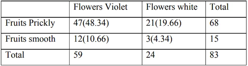
- The following data are observed for hybrids of Datura.
- Flowers violet, fruits prickly = 47
- Flowers violet, fruits smooth = 12
- Flowers white, fruits prickly = 21
- Flowers white, fruits smooth = 3
- Using chi-square test, find the association between colour of flowers and character of fruits.
Solution:
- H0: The two attributes colour of flowers and fruits are independent.
- We cannot use Yate’s correction for continuity based on observed values.
- If only expected frequency less than 5, we use Yates’s correction for continuity.
- The test statistic is
The figures in the brackets are the expected frequencies
- Calculated value of χ2 = 0.28
- Table value of χ2 for (2-1) (2-1) = 1 d.f. is 3.84
- Calculated value of χ2 < table value of χ2, H0 is accepted and hence we conclude that colour of flowers and character of fruits are not associated. Since the calculated chi-square (0.28) is much smaller than the critical value (3.84), there is no evidence that flower colour and fruit character are linked in these Datura hybrids.
Summary Table
| Concept | Key Point | Exam Tip |
|---|---|---|
| Type | Non-parametric (distribution-free) test | No assumption about population distribution |
| Discoverer | Helmert (1876), independently Karl Pearson (1900) | |
| Range | 0 to ∞ | Never negative (sum of squares) |
| Data type | Enumeration (count) data — discrete variables | t-test and Z-test use measurement data |
| Formula | χ² = ∑(O-E)²/E | O = observed, E = expected |
| d.f. (goodness of fit) | n - 1 | n = number of classes |
| d.f. (contingency table) | (m-1)(n-1) | m rows, n columns |
| If O = E | χ² = zero | Perfect agreement |
| Validity condition 1 | N > 50 | Total frequency must be large |
| Validity condition 2 | Expected frequency ≥ 5 in each cell | Pool adjacent classes if < 5 |
| Yates correction | For 2x2 table when expected frequency < 5 | Add 0.5 to smallest cell |
| Agricultural use | Mendelian ratios, genetic linkage, attribute independence | Most tested application |
| Application | What It Tests |
|---|---|
| Goodness of fit | Do observed frequencies match theoretical ratios? |
| Independence | Are two attributes (e.g., flower colour, leaf shape) independent? |
| Homogeneity of variances | Are variances from multiple samples equal? |
| Genetic linkage | Are two genes inherited independently? |
TIP
Mnemonic for chi-square validity: “Fifty-Five” — Total N > 50 and every expected cell ≥ 5.
Summary Cheat Sheet
| Concept / Topic | Key Details |
|---|---|
| Chi-square test | Non-parametric (distribution-free) test |
| Discovered by | Helmert (1876); independently Karl Pearson (1900) |
| Range | 0 to ∞ (sum of squares, never negative) |
| Data type | Enumeration (count) data — discrete variables |
| Formula | χ² = ∑(O - E)²/E where O = observed, E = expected |
| If O = E | χ² = zero (perfect agreement) |
| d.f. (goodness of fit) | n - 1 (n = number of classes) |
| d.f. (contingency table) | (m - 1)(n - 1) for m rows, n columns |
| d.f. for 2x2 table | (2-1)(2-1) = 1 |
| Validity: total N | Must be > 50 |
| Validity: expected freq | Each cell must be ≥ 5; if < 5, pool adjacent classes |
| Yates correction | For 2x2 table when expected frequency < 5; add 0.5 to smallest cell |
| Expected frequency | (Row total x Column total) / Grand total |
| Goodness of fit | Tests if observed matches theoretical ratios (e.g., 9:3:3:1) |
| Independence test | Tests if two attributes are independent |
| Genetic linkage | Tests if two genes are inherited independently |
| Homogeneity of variances | Tests if variances from multiple samples are equal |
| Measurement data | Obtained by actual measurement (height, weight) — use t/Z test |
| Enumeration data | Obtained by counting — use χ² test |
| Mendelian ratios | Most tested agricultural application of chi-square |
| Parametric tests | Z, t, F — require distributional assumptions |
| Non-parametric | χ² — no assumptions about population distribution |
Knowledge Check
Take a dynamically generated quiz based on the material you just read to test your understanding and get personalized feedback.
Lesson Doubts
Ask questions, get expert answers