🧚🏼♂️ Latin Square Design (LSD)
Layout, mathematical model, ANOVA, two-way error control, treatment range (5-12), row-column blocking — for fields with fertility gradients in two directions
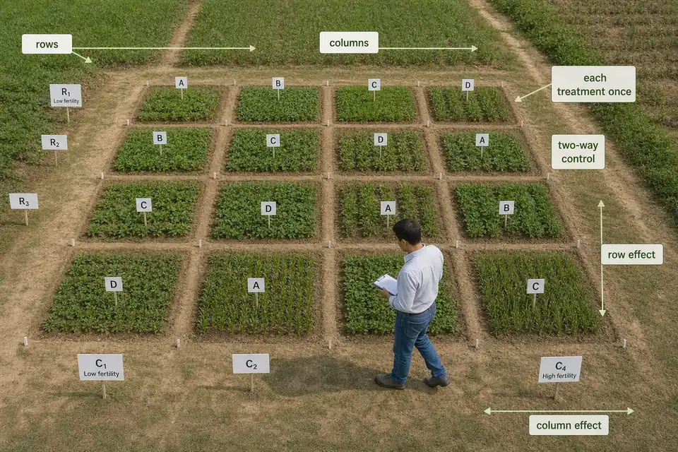
Imagine a field where soil fertility varies both north-south (due to slope) and east-west (due to proximity to a canal). RBD can control variation in only one direction. The Latin Square Design handles both by arranging treatments so that each appears exactly once in every row and every column — much like a Sudoku puzzle for treatments, ensuring the fairest possible comparison.
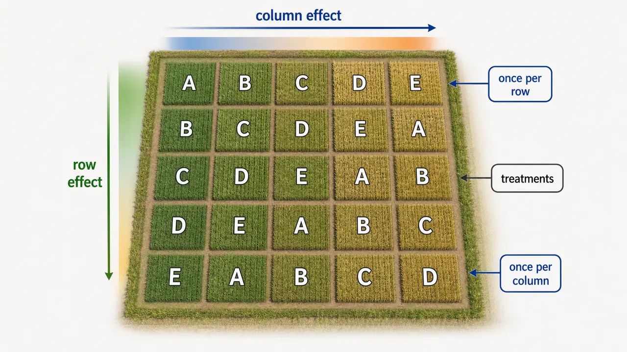
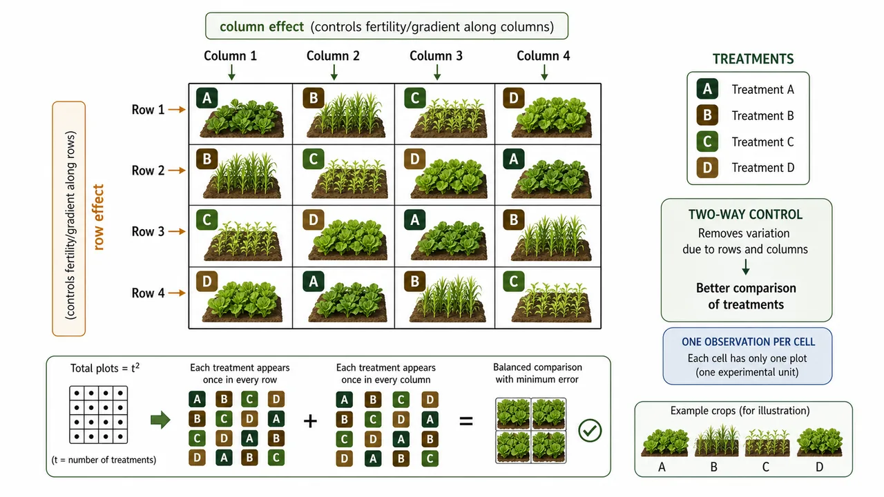
- When the experimental material is divided into rows and columns and the treatments are allocated such that each treatment occurs only once in a row and once in a column, the design is known as latin square design. In this design eliminating fertility variations consists in an experimental layout which will control variation in two perpendicular direction. This is the defining feature of LSD -- it accounts for two sources of heterogeneity simultaneously (e.g., soil fertility varying both north-south and east-west across a field).
- Latin square designs are normally used in experiments where it is required to remove the heterogeneity of experimental material in two directions. While RBD controls variation in one direction (through blocks), LSD goes a step further by controlling variation in both row and column directions.
Simple idea:
Use LSD when the field varies in two directions at the same time. Rows control one direction, columns control the other.
Pro Content Locked
Upgrade to Pro to access this lesson and all other premium content.
Charged once for one year · ₹1188 total
Save ₹100/month vs ₹2388/year launch price
- All Agriculture & Banking Courses
- AI Lesson Questions (100/day)
- AI Doubt Solver (50/day)
- Glows & Grows Feedback (30/day)
- AI Section Quiz (20/day)
- 22-Language Translation (100/day)
- Recall Questions (20/day)
- AI Quiz (15/day)
- AI Quiz Paper Analysis (100/day)
- AI Step-by-Step Explanations (100/day)
- Spaced Repetition Recall (FSRS)
- AI Tutor
- Immersive Text Questions
- Audio Lessons — Hindi & English
- Mock Tests & Previous Year Papers
- Summary & Mind Maps
- XP, Levels, Leaderboard & Badges
- Generate New Classrooms
- Voice AI Teacher (AgriDots Live)
- AI Revision Assistant
- Knowledge Gap Analysis
- Interactive Revision (LangGraph)
🔒 Secure one-time yearly payment via Razorpay · No hidden fees
Imagine a field where soil fertility varies both north-south (due to slope) and east-west (due to proximity to a canal). RBD can control variation in only one direction. The Latin Square Design handles both by arranging treatments so that each appears exactly once in every row and every column — much like a Sudoku puzzle for treatments, ensuring the fairest possible comparison.
- When the experimental material is divided into rows and columns and the treatments are allocated such that each treatment occurs only once in a row and once in a column, the design is known as latin square design. In this design eliminating fertility variations consists in an experimental layout which will control variation in two perpendicular direction. This is the defining feature of LSD -- it accounts for two sources of heterogeneity simultaneously (e.g., soil fertility varying both north-south and east-west across a field).
- Latin square designs are normally used in experiments where it is required to remove the heterogeneity of experimental material in two directions. While RBD controls variation in one direction (through blocks), LSD goes a step further by controlling variation in both row and column directions.
Simple idea:
Use LSD when the field varies in two directions at the same time. Rows control one direction, columns control the other.
- This design requires that the number of replications (rows) equal the number of treatments. In LSD the number of rows and number of columns are equal. Hence the arrangement will form a square. NABARD Mains-2020. This square arrangement is where the name "Latin Square" comes from -- each treatment letter (A, B, C...) appears exactly once in every row and every column, much like a Sudoku puzzle for treatments.
TIP
Easy memory rule:
- rows = columns = treatments
- each treatment appears once in every row
- each treatment appears once in every column
Layout of LSD
- In this design the number of rows is equal to the number of columns and it is equal to the number of treatments. Thus, in case of 'm' treatments, there have to be m x m = m2 experimental units (plots) arranged in a square so that each row as well as each column contain 'm' plots.
- The 'm' treatments are then allocated at random to these rows and columns in such a way that every treatment occurs once and only once in each row and each column such a layout is known as m x m L.S.D. and is extensively used in agricultural experiments.
- The minimum and maximum number of treatments required for layout of LSD is 5 to 12. Because the minimum error degree of freedom should be 12. Should not be used for less than 5 treatments. With fewer than 5 treatments, the error degrees of freedom become too small (e.g., a 4x4 LSD has only (4-1)(4-2) = 6 error d.f., which is inadequate). With more than 12 treatments, the design becomes impractically large, requiring 144+ plots.
- In LSD the treatments are usually denoted by alphabets like A, B, C...etc. For a latin square with five treatments the arrangement may be as follows:
| Square I | Square II | ||||||||
|---|---|---|---|---|---|---|---|---|---|
| A | B | C | D | E | A | B | C | D | E |
| B | A | E | C | D | B | A | D | E | C |
| C | D | A | E | B | C | E | A | B | D |
| D | E | B | A | C | D | C | E | A | B |
| E | C | D | B | A | E | D | B | C | A |
Mathematical Model
yijk = μ + αi + βj + γk + ξijk
- i = j = k = 1,2,......
- Where
- Yijk denote the response from the unit (plot) in the ith row, jth column and receiving the kth treatment.
- μ = general mean effect -- the overall average response across the entire experiment.
- αi = ith row effect -- accounts for the systematic variation between rows.
- βj = jth column effect -- accounts for the systematic variation between columns.
- γk = kth treatment effect -- the actual effect of the treatment we want to measure.
- ξijk = error effect -- the remaining random variation after accounting for rows, columns, and treatments.
- We know that total variation =
Variation due to rows + variation due to columns + Variation due to treatments + variation due to error
This partitioning is the core of LSD analysis. By removing row and column variation from the total, the error term becomes smaller, making it easier to detect real treatment differences.
That is why LSD is usually more precise than RBD when the assumptions fit the field situation.
- Null hypothesis (H0) = There is no significant difference between Rows, Columns and Treatment effects.
- i.e.
- H01: α1 = α2 = ............ αm
- H02: β1 = β2 = ......... = βm and
- H03: γ1 = γ2 = .................... = γm
- The steps in the analysis of the data for verifying the null hypothesis are: Different component variations can be calculated as follows:
ANOVA
| Sources | D.F. | S.S. | M.S. | F-cal. value | F-table value at 5% LOS |
|---|---|---|---|---|---|
| Rows | m - 1 | RSS | RMS = RSS / (m - 1) | F_R = RMS / EMS | F_R[m - 1, (m - 1)(m - 2)] |
| Columns | m - 1 | CSS | CMS = CSS / (m - 1) | F_C = CMS / EMS | same as above |
| Treatments | m - 1 | Tr.S.S. | TMS = Tr.S.S. / (m - 1) | F_T = TMS / EMS | same as above |
| Error | (m - 1)(m - 2) | ESS | EMS = ESS / ((m - 1)(m - 2)) | - | - |
| Total | m^2 - 1 | TSS | - | - | - |
- If calculate value of F(Tr) < table value of Fat 5% LOS, H0 is accepted and hence we may conclude that there is no significance difference between treatment effects.
- If calculate value of F(Tr) > table value of F at 5% LOS, H0 is rejected and hence we may conclude that there is significance difference between treatments effects.
- If the treatments are significantly different, the comparison of the treatments is carried out on the basis of Critical Difference (C.D.). The C.D. value is used to perform pairwise comparisons between treatment means -- if the difference between any two treatment means exceeds the C.D., those treatments are declared significantly different.
Exam interpretation:
A significant treatment F-value in LSD means the treatment means are not all equal even after controlling row and column variation.
Advantages of Latin Square Design
- With two way grouping or stratification LSD controls more of the variation than C.R.D. or R.B.D. This makes LSD the most precise among the three basic designs when the experimental material has variation in two directions.
- L.S.D. is an incomplete 3-way layout. Its advantage over complete 3-way layout is that instead of m3 experimental units only m2 units are needed.
- Thus a 4 x 4 L.S.D. results in saving of 64 - 16 = 48 observations over a complete 3-way layout.
- The statistical analysis is simple though slightly complicated than for R.B.D. Even with missing data the analysis remains relatively simple.
- More than one factor can be investigated simultaneously.
- The missing observations can be analysed by using missing plot technique.
- Three-way classification and two-way control of error. This means the data is classified three ways (by row, column, and treatment), and the error is controlled in two directions (rows and columns).
- This design is used when fertility gradient is in two directions.
Number of replications = Number of treatments.
Number of rows = Number of columns = Number of treatments.
- Randomization of treatments is done in such a way that each treatment occurs once and only once in each row and each column. This balanced arrangement ensures that every treatment is exposed to the full range of row and column conditions, making the treatment comparisons fair.
- Error degree of freedom in LSD: (n - 1) x (n - 2). For example, with 5 treatments, the error d.f. = (5-1) x (5-2) = 4 x 3 = 12.
Quick Comparison: CRD vs RBD vs LSD
| Feature | CRD | RBD | LSD |
|---|---|---|---|
| Classification | One-way | Two-way | Three-way |
| Error control | None | One-way (blocks) | Two-way (rows + columns) |
| Principles used | Replication, Randomization | All three | All three |
| Best for | Lab/homogeneous material | Field (1-direction gradient) | Field (2-direction gradient) |
| Treatments | Any number | Up to 20 | 5 to 12 |
| Error d.f. | N - k | (r-1)(k-1) | (n-1)(n-2) |
| Replications | Flexible (can be unequal) | Equal across treatments | = Number of treatments |
Summary Cheat Sheet
| Concept / Topic | Key Details |
|---|---|
| LSD | Latin Square Design — controls variation in two directions |
| Classification | Three-way (row, column, treatment), two-way control |
| Principles used | All three — replication, randomisation, local control |
| Best for | Field with fertility gradient in two perpendicular directions |
| Square arrangement | Rows = Columns = Treatments (forms an m x m square) |
| Replications | = Number of treatments |
| Treatment range | 5 to 12 (min error d.f. must be ≥ 12) |
| Error d.f. | (n-1)(n-2) where n = number of treatments |
| Mathematical model | y_ijk = μ + α_i + β_j + γ_k + ξ_ijk |
| α_i | Row effect |
| β_j | Column effect |
| γ_k | Treatment effect |
| Total variation | Row SS + Column SS + Treatment SS + Error SS |
| Savings over 3-way | m² units instead of m³ (e.g., 4x4 saves 48 observations) |
| More precise than | CRD and RBD — controls more variation |
| Incomplete 3-way layout | Only m² experimental units needed |
| Critical Difference | Used for pairwise comparisons when F-test is significant |
| Missing data | Can be analysed using missing plot technique |
| < 5 treatments | Not suitable (too few error d.f.) |
| > 12 treatments | Impractically large (requires 144+ plots) |
| Each treatment | Appears once in every row and every column |