😵💫 Completely Randomised Design (CRD)
Layout, mathematical model, ANOVA table, critical difference, advantages and disadvantages — the simplest experimental design for homogeneous material
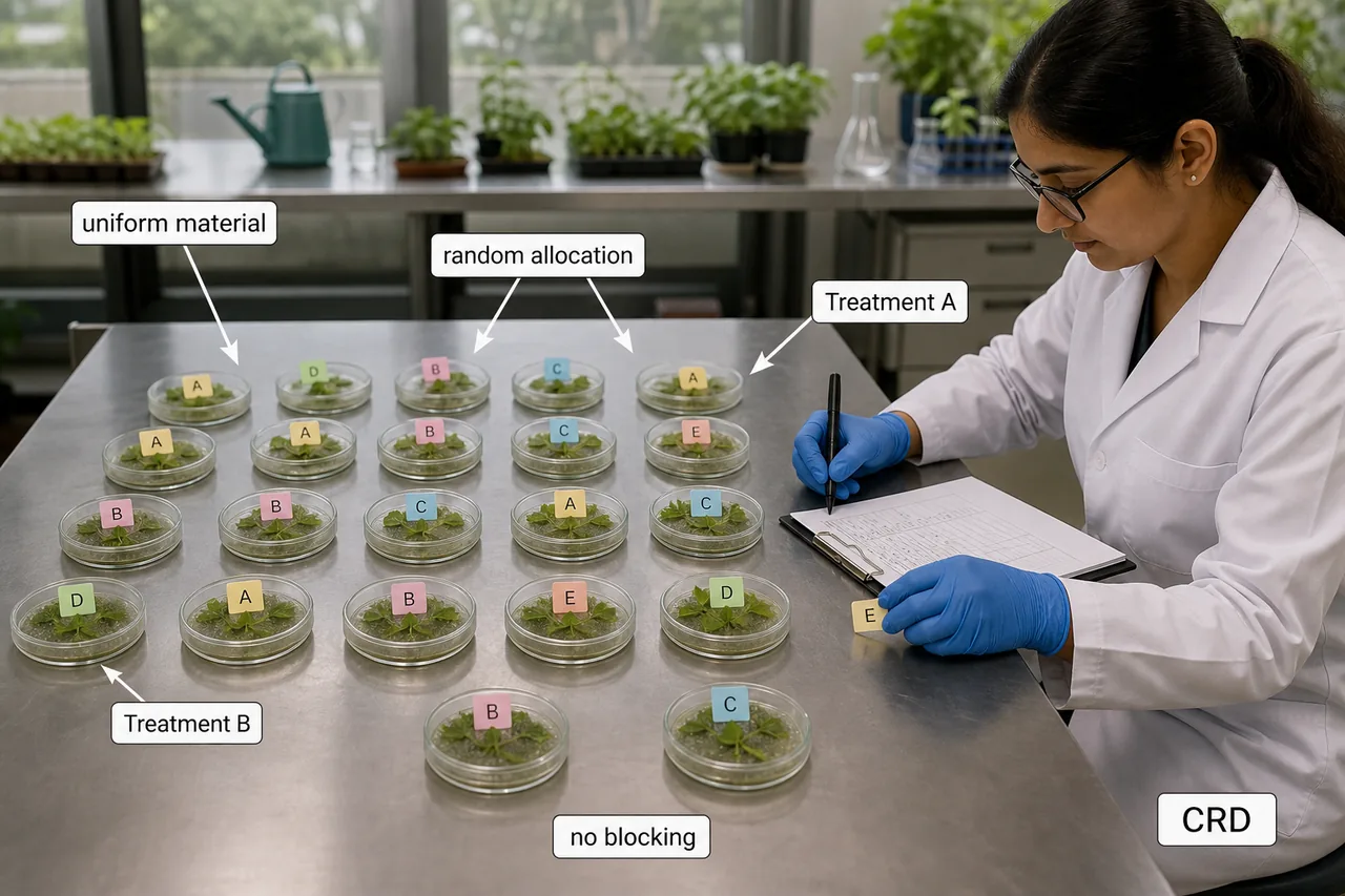
In a plant pathology laboratory, a researcher wants to compare the efficacy of five fungicides on disease control. Since all petri dishes in the lab have identical growing conditions, there is no need for blocking. She simply randomises the five treatments across 20 petri dishes — this is the Completely Randomised Design, the simplest and most straightforward experimental layout.
-
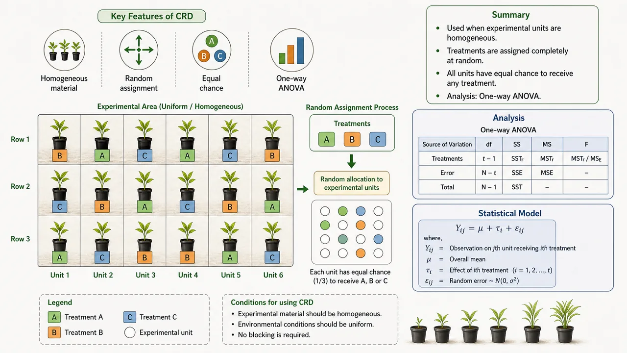
The CRD is the simplest of all the designs. In this design, treatments are allocated at random to the experimental units over the entire experimental material. In case of field experiments, the whole field is divided into a required number of plots equal size and then the treatments are randomized in these plots. Thus the randomization gives every experimental unit an equal probability of receiving the treatment. This means there is no grouping or blocking of experimental units -- the entire experimental area is treated as one homogeneous unit.
Pro Content Locked
Upgrade to Pro to access this lesson and all other premium content.
Charged once for one year · ₹1188 total
Save ₹100/month vs ₹2388/year launch price
- All Agriculture & Banking Courses
- AI Lesson Questions (100/day)
- AI Doubt Solver (50/day)
- Glows & Grows Feedback (30/day)
- AI Section Quiz (20/day)
- 22-Language Translation (100/day)
- Recall Questions (20/day)
- AI Quiz (15/day)
- AI Quiz Paper Analysis (100/day)
- AI Step-by-Step Explanations (100/day)
- Spaced Repetition Recall (FSRS)
- AI Tutor
- Immersive Text Questions
- Audio Lessons — Hindi & English
- Mock Tests & Previous Year Papers
- Summary & Mind Maps
- XP, Levels, Leaderboard & Badges
- Generate New Classrooms
- Voice AI Teacher (AgriDots Live)
- AI Revision Assistant
- Knowledge Gap Analysis
- Interactive Revision (LangGraph)
🔒 Secure one-time yearly payment via Razorpay · No hidden fees
In a plant pathology laboratory, a researcher wants to compare the efficacy of five fungicides on disease control. Since all petri dishes in the lab have identical growing conditions, there is no need for blocking. She simply randomises the five treatments across 20 petri dishes — this is the Completely Randomised Design, the simplest and most straightforward experimental layout.
-
The CRD is the simplest of all the designs. In this design, treatments are allocated at random to the experimental units over the entire experimental material. In case of field experiments, the whole field is divided into a required number of plots equal size and then the treatments are randomized in these plots. Thus the randomization gives every experimental unit an equal probability of receiving the treatment. This means there is no grouping or blocking of experimental units -- the entire experimental area is treated as one homogeneous unit.
-
In field experiments there is generally large variation among experimental plots due to soil heterogeneity. Hence, CRD is not preferred in field experiments. Since CRD has no mechanism to account for soil variability (no blocks), the differences caused by uneven soil fertility get mixed into the error term, making it harder to detect real treatment differences.
-
In laboratory experiments and green house studies, it is easy to achieve homogeneity of experimental materials. Therefore, CRD is most useful in such experiments. In a laboratory, conditions like temperature, humidity, and lighting can be tightly controlled, making the experimental units very uniform -- exactly the condition CRD requires to work well.
Rule of thumb:
Use CRD when the experimental material is uniform enough that blocking is unnecessary.
Layout of CRD
- The placement of the treatments on the experimental units along with the arrangement of experimental units is known as the layout of an experiment. For example, suppose that there are 5 treatments A, B, C, D and E. Each with 4 replications, we need 20 experimental units. Here, since the number of units is 20, a two digit random number of table will be consulted and a series of 20 random numbers will be taken excluding those which are greater than 20.
- Suppose, the random numbers are 4, 18, 2, 14, 3, 7, 13, 1, 6, 10, 17, 20, 8, 15, 11, 5, 9, 12, 16, 19. After this the plots will be serially numbered and the treatment A will be allotted to the plots bearing the serial numbers 4, 18, 2, 14 and so on. This process of using random number tables ensures that the allocation is free from any personal bias of the researcher.
| 1 | 2 | 3 | 4 | 5 |
|---|---|---|---|---|
| B | A | B | A | D |
| 6 | 7 | 8 | 9 | 10 |
| C | B | D | E | C |
| 11 | 12 | 13 | 14 | 15 |
| D | E | B | A | D |
| 16 | 17 | 18 | 19 | 20 |
| E | C | A | E | C |
This layout shows the main idea of CRD: treatments are scattered purely at random over all units, without first forming blocks.
Statistical analysis
- Let us suppose that there are 'k' treatments applied to 'r' plots. These can be represented by the symbols as follows:
| Treatments | Replications | Totals | Means |
|---|---|---|---|
| t_1 | y_11, y_12, ..., y_1r | T_1 | \bar{T}_1 |
| t_2 | y_21, y_22, ..., y_2r | T_2 | \bar{T}_2 |
| \vdots | \vdots | \vdots | \vdots |
| t_i | y_i1, y_i2, ..., y_ir | T_i | \bar{T}_i |
| \vdots | \vdots | \vdots | \vdots |
| t_k | y_k1, y_k2, ..., y_kr | T_k | \bar{T}_k |
| Grand total | - | G.T. | - |
Mathematical Model
yij = μ + αi + ξij
- i = 1,2,....k & j = 1,2,......r
- Where, yij is the jth replication of the ith treatment
- μ = general mean effect (Common in all designs). This represents the overall average response across all treatments and replications.
- αi = the effect due to ith treatment. This is the deviation of the i-th treatment mean from the overall mean.
- ξij = error effect. This captures all uncontrolled random variation in the experiment.
- Source of Variability in CRD:
- Due to treatment
- Error
Notice that in CRD there is no blocking. So the total variation is partitioned into just two components: treatment variation and error variation.
- The null hypothesis can be verified by applying the ANOVA procedure. The steps involved in this procedure are as follows:
- N -- Number of observations
ANOVA table
| Sources of variation | D.F. | S.S. | M.S. | F-cal. value | F-table value |
|---|---|---|---|---|---|
| Treatments | k - 1 | Tr.S.S. | TMS = Tr.S.S. / (k - 1) | F_t = TMS / EMS | F[k - 1, N - k] at \alpha% LOS |
| Error | N - k | ESS | EMS = ESS / (N - k) | - | - |
| Total | N - 1 | TSS | - | - | - |
- If the calculated value of F > table vale of F, H0 is rejected. Then the problem is to know which of the treatment means are significantly different. When the F-test tells us that at least one treatment is different, we need a follow-up comparison to identify exactly which treatments differ from each other.
- For this, we calculate critical difference (CD):
- CD = SED x t -- table value for error d.f. at 5% LOS.
- Where,
- SED = Standard Error of Difference between the Treatments
- The treatment means are arranged first in descending order of magnitude. If the difference between the two-treatment means is less than CD value, it will he declared as non-significant otherwise significant. This pairwise comparison allows us to rank treatments and identify which ones are statistically superior.
Meaning of CD:
CD tells us the minimum difference required between two treatment means before we call that difference statistically real.
Advantages and disadvantages of CRD
- It is regarded as one-way classification and no-way control or elimination. This means the data is classified only by treatments (one-way), and there is no attempt to control or eliminate any known source of variation through blocking.
- This design is most commonly used in laboratory experiments such as in Ag. Chemistry, plant pathology, and animal experiments where the experimental material is expected to be homogeneous.
- Applied when the experimental material is limited and homogenous, such as the soil in Pot culture experiments. However, in greenhouse experiments care has to be taken with regard to sunshade, accessibility of air along and across the bench before conducting the experiment.
In one line:
CRD is best when units are already similar, so randomisation alone is enough.
-
Any number of replications and treatments can be used. The number of replications may vary from treatment to treatment. This flexibility in replication is a unique advantage of CRD -- in RBD and LSD, every treatment must have the same number of replications.
-
The analysis remains simple even if information on some units are missing.
-
This design provides maximum number of degrees of freedom for the estimation of error than the other designs. Since there are no blocks, the degrees of freedom that would have gone to blocks in other designs are added to the error, giving a more precise estimate of experimental error (provided the material is homogeneous).
-
The only drawback with this design is that when the experimental material is heterogeneous, the experimental error would be inflated and consequently the treatments are less precisely compared. The only way to keep the experimental error under control is to increase the number of replications thereby increasing the degrees of freedom for error.
-
Local control not used in CRD. This is the key distinction from RBD and LSD, which employ blocking to reduce error.
-
Error degree of freedom in CRD: N - k. Where N is the total number of observations and k is the number of treatments.
NOTE
CRD Summary: One-way classification, no-way control, simplest design, best for homogeneous material (lab experiments), error d.f. = N - k.
Applications
- CRD is most useful in laboratory technique and methodological studies. Ex: in physics, chemistry, in chemical and biological experiments, in some greenhouse studies etc.
- CRD is also recommended in situations where an appreciable fraction of units is likely to be destroyed or fail to respond. Since CRD allows unequal replication, losing some units does not create the complications it would in balanced designs like RBD or LSD.
- CRD can be used with both equal and unequal number of repetitions.
Summary Cheat Sheet
| Concept / Topic | Key Details |
|---|---|
| CRD | Completely Randomised Design — simplest experimental design |
| Classification | One-way classification, no-way control/elimination |
| Principles used | Replication + Randomisation only (no local control) |
| Best for | Laboratory, greenhouse, homogeneous material |
| Not preferred for | Field experiments (soil heterogeneity inflates error) |
| Mathematical model | y_ij = μ + α_i + ξ_ij |
| μ | General mean effect (common to all designs) |
| α_i | Effect of i-th treatment |
| ξ_ij | Error effect (uncontrolled variation) |
| Error d.f. | N - k (N = total observations, k = treatments) |
| Replications | Can be unequal across treatments (unique advantage) |
| Max error d.f. | Provides maximum error d.f. compared to RBD/LSD |
| Missing data | Analysis remains simple even with missing observations |
| Layout | Random allocation using random number tables |
| ANOVA | Total SS = Treatment SS + Error SS |
| Critical Difference | CD = SED x t-table value; identifies which means differ |
| SED formula | \sqrt{(2 \times \text{Error MS}) / r} |
| Drawback | If material is heterogeneous, error inflates → less precision |
| Remedy for heterogeneity | Increase number of replications |
| Applications | Chemistry, pathology, pot culture, animal experiments |
| Compared to RBD | RBD is more efficient due to local control |